Tree-Based AI Beyond Prediction:

Individual Variable Priority for Precision Insights

Min Lu (presenter) and Hemant Ishwaran
University of Miami

South Florida ASA Symposium

Why care about individual importance?

Average (global) importance can miss heterogeneity
e.g. \(y_i = \beta_0 + \beta_1 x_{i1} + \beta_2 x_{i2} + \dots + \beta_p x_{ip} + \varepsilon_i\)
Precision decisions need patient-specific drivers
We want sensitivity: “how much does a tiny nudge in \(x^{(s)}\) change my outcome?”

Global vs individual importance schematic

We rely on Artificial Intelligence (AI)

Neural net-based AI \(\quad\) Tree-based AI

Neuron activation: Composes nonlinear functions via weighted layers
Deep neural nets, CNNs: Optimized through gradient descent

Decision Trees: Rule-based “if–else” splits; intuitive to explain
Random Forests, Boosting: Ensembles that improve stability and accuracy

From population to individual

Population: “What matters on average?” (Breiman’s permutation importance)
Individual: “What matters for this case?”

Let \(\def\grad{{ \nabla}}\def\x{{\bf x}}\def\xs#1{x^{(#1)}}\psi(\x) = \mathbb{E}(\phi(Y) | \x)\) be the unknown target function for the feature vector \(\x = (\xs{1}, \ldots, \xs{p})^T\), where \(Y\) is the outcome and the choice of \(\phi\) depends on the specific problem

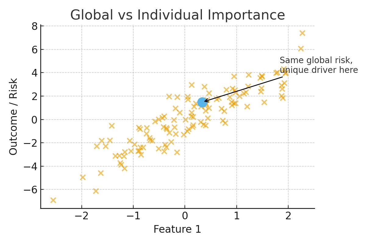
iVarPro defines individual importance as the local gradient: \[ \grad \psi(\x) = \left(\frac{\partial \psi(\x)}{\partial \xs{1}}, \ldots, \frac{\partial \psi(\x)}{\partial \xs{p}}\right)^T := \left(g^{(1)}(\x), \ldots, g^{(p)}(\x)\right)^T \] The values \(g^{(s)}(\x)\) represent the individual variable importance for features \(\xs{s}, s = 1, \ldots, p\)

Intuition: gradient = sensitivity to small changes in \(x^{(s)}\) at this \(\x\)

Core idea in one picture

Use tree rules to define a local region \(R\) around a point
Release the constraint on one variable \(x^{(s)}\) to get variation only along that axis

\(\quad\quad\) Random Forest

Tree partitions and release region schematic

Variable Priority (VarPro) rules

rule region schematic

Core idea in one picture

Use tree rules (VarPro) to define a local region \(R\) around a point
Release the constraint on one variable \(x^{(s)}\) to get variation only along that axis
Fit a tiny local linear regression to get the slope = gradient
Average over many rules to obtain individual variable priority (iVarPro) score

Tree partitions and release region schematic

Why not just SHAP or LIME?

SHAP (Shapley Additive Explanations) or LIME (Local Interpretable Model-Agnostic Explanations) depend on the fitted model and a background distribution
Perturbations can create unrealistic points
iVarPro stays model-independent, uses observed data only, and targets directional derivatives directly

Working theory: when the surface \(\psi(x)\) is smooth locally, these tiny local regressions recover gradients well

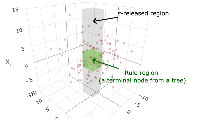
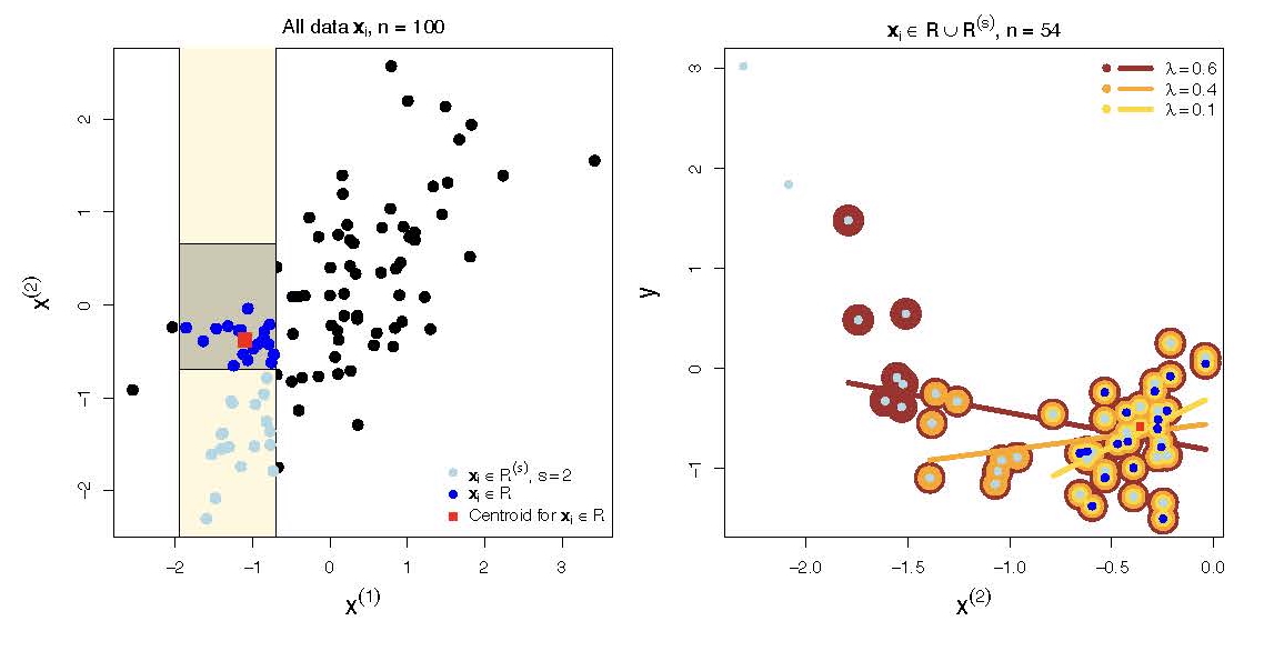
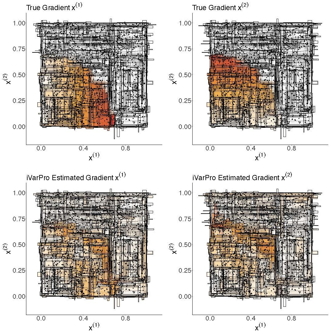
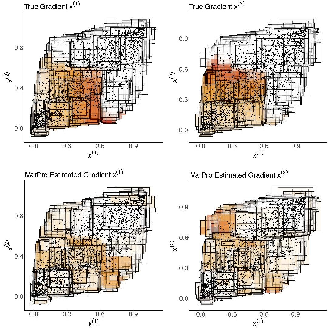
VarPro: using rules to obtain local gradients

The importance of a variable \(s \in \{1, \ldots, p\}\) is assessed by comparing estimates within a rule’s region \(R\) to those in its corresponding release region, defined as the region \(R\) expanded where constraints on \(\xs{s}\) are removed [1]

Let \(\x_0 := \x_0(R)\) denote the centroid of \(R\), and assign its gradient to all cases in \(R\). To define the gradient at \(\x_0 = (x_0^{(1)},\ldots,x_0^{(p)})^T\) along coordinate \(s\), let \(\psi_R^{(s)}(z)\) represent the evaluation of \(\psi\) at \(\x_0\), with the \(s\)-th coordinate perturbed by an increment \(z\): \[ \psi_R^{(s)}(z) = \psi(x_0^{(1)},\ldots,x_0^{(s-1)},x_0^{(s)}+z,x_0^{(s+1)},\ldots,x_0^{(p)}) \] By construction, \(\psi_R^{(s)}(0) = \psi(\x_0)\), and the gradient of \(\psi\) at \(\x_0\) along coordinate \(s\) is formally given by \[ g_R^{(s)} := g_R^{(s)}(\x_0) =\lim_{z\rightarrow 0} \frac{\psi_R^{(s)}(z)-\psi_R^{(s)}(0)}{z} \]

Gradient estimation via local linear regression

To estimate the gradient, we employ a local linear regression model. In small regions around \(\x_0(R)\) along the coordinate direction \(s\), we approximate \(\psi\) using the linear model: \[ \psi_R^{(s)}(z) = \psi_R^{(s)}(0) + z g_R^{(s)} \] Given training data \((\x_1, y_1),\ldots,(\x_n, y_n)\), we regress \(\{y_i\}\) on the \(s\)-coordinate features \(\{x_i^{(s)}\}\) using an intercept-slope model based on data local to \(R\). The gradient \(g_R^{(s)}\) is estimated using the least squares estimate of the slope

Standardized covariates

To systematically control the extent of this expansion, we introduce an index \(\scriptsize \def\l{\lambda} \def\psihat{\widehat{\psi}} \def\ghat{\widehat{g}} \def\bhat{\widehat{\beta}} 0 \le \l \le \l_0\) that determines the proportion of individuals selected from the release region \(\scriptsize R^{(s)}\). Larger values of \(\scriptsize \l\) correspond to a greater number of included individuals. The expanded region is then defined as \(\scriptsize R(s,\l) = R \cup R_\l^{(s)}\), where \(\scriptsize R_\l^{(s)}\) is a restricted subset of \(\scriptsize R^{(s)}\) determined by \(\scriptsize \l\)

we center \(\scriptsize x_i^{(s)}\) at the centroid value \(\scriptsize x_0^{(s)}(R)\) and then scale it to have unit length, denoting the transformed values by \(\scriptsize z_i^{(s)}\):

\[ \scriptsize z_i^{(s)} = \frac{x_i^{(s)} - x_0^{(s)}(R)} {\sqrt{\displaystyle\sum_{\x_j\in R(s,\lambda)}(x_j^{(s)} - x_0^{(s)}(R))^2}} %\quad \x_i\in R(s,\lambda) \]

The local gradient is estimated via least squares regression using the data \(\scriptsize \{z_i^{(s)},\psihat(\x_i)\}\) within \(\scriptsize R(s,\lambda)\): \[ \scriptsize \psihat(\x_i) = \alpha_R^{(s)} + z_i^{(s)} \beta_R^{(s)} + \varepsilon_i, \quad \x_i \in R(s,\lambda) \] The least-squares slope is then used as the local gradient estimate: \(\scriptsize \ghat_R^{(s)}:=\bhat_R^{(s)}\)

Cross-Validation for optimizing the fit

For a given \(\scriptsize \def\l{\lambda} \def\fhat{\widehat{f}} \l\), the Predicted Residual Sum of Squares (PRESS) statistic is computed as follows. The leave-one-out (LOO) residual for observation \(\scriptsize i\) is: \[ {\tiny e_i = \psihat(\x_i) - \fhat^{(-i)}(z_i^{(s)}), } \] where \(\scriptsize \fhat^{(-i)}(z_i^{(s)})\) is the least squares predicted value at \(\scriptsize z_i^{(s)}\) when the \(\scriptsize i\)-th observation is excluded from the regression fit. The PRESS statistic is then given by: \[ {\tiny \text{PRESS}(s,\l) = \frac{1}{|R(s,\l)|} \sum_{i\in R(s,\l)} e_i^2 } \] Since local regression follows a linear model, the PRESS statistic simplifies in terms of leverage values \(\scriptsize h_i\): \(\scriptsize e_i = \frac{\psihat(\x_i) - \fhat(z_i^{(s)})}{1 - h_i},\) where \(\scriptsize h_i\) is the leverage for \(\scriptsize z_i^{(s)}\) and \(\scriptsize \fhat\) is the least squares predictor. Thus, the PRESS statistic can be rewritten as: \[{\tiny \text{PRESS}(s,\l) = \frac{1}{|R(s,\l)|} \sum_{i\in R(s,\l)} \left( \frac{\psihat(\x_i) - \fhat(z_i^{(s)})}{1 - h_i} \right)^2 } \] The optimal \(\scriptsize \l^*=\text{argmin}_\l \text{PRESS}(s,\l)\) is selected

iVarPro pipeline

Build VarPro rules (randomized trees)
→ small rectangular regions (R)
For each feature \(s\) and rule \(R\):
- Release \(x^{(s)}\) to form \(R^{(s)}(\lambda)\)
- Standardize \(x^{(s)}\) around the region centroid
- Regress ((x)) on standardized \(x^{(s)}\), choose \(\lambda\) by PRESS (LOO)
- Slope \(\Rightarrow \widehat{g}^{(s)}_R\)
For case \(x_i\): average \(\widehat{g}^{(s)}_R\) over all rules containing \(x_i\)

Tip: \(\widehat{\psi}\) from RF/GBM/XGBoost smooths noise → better local slopes

Simulation contour gradients

Synthetic experiments

Model 1 is generated according to a piecewise function:

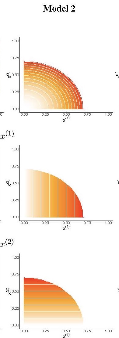
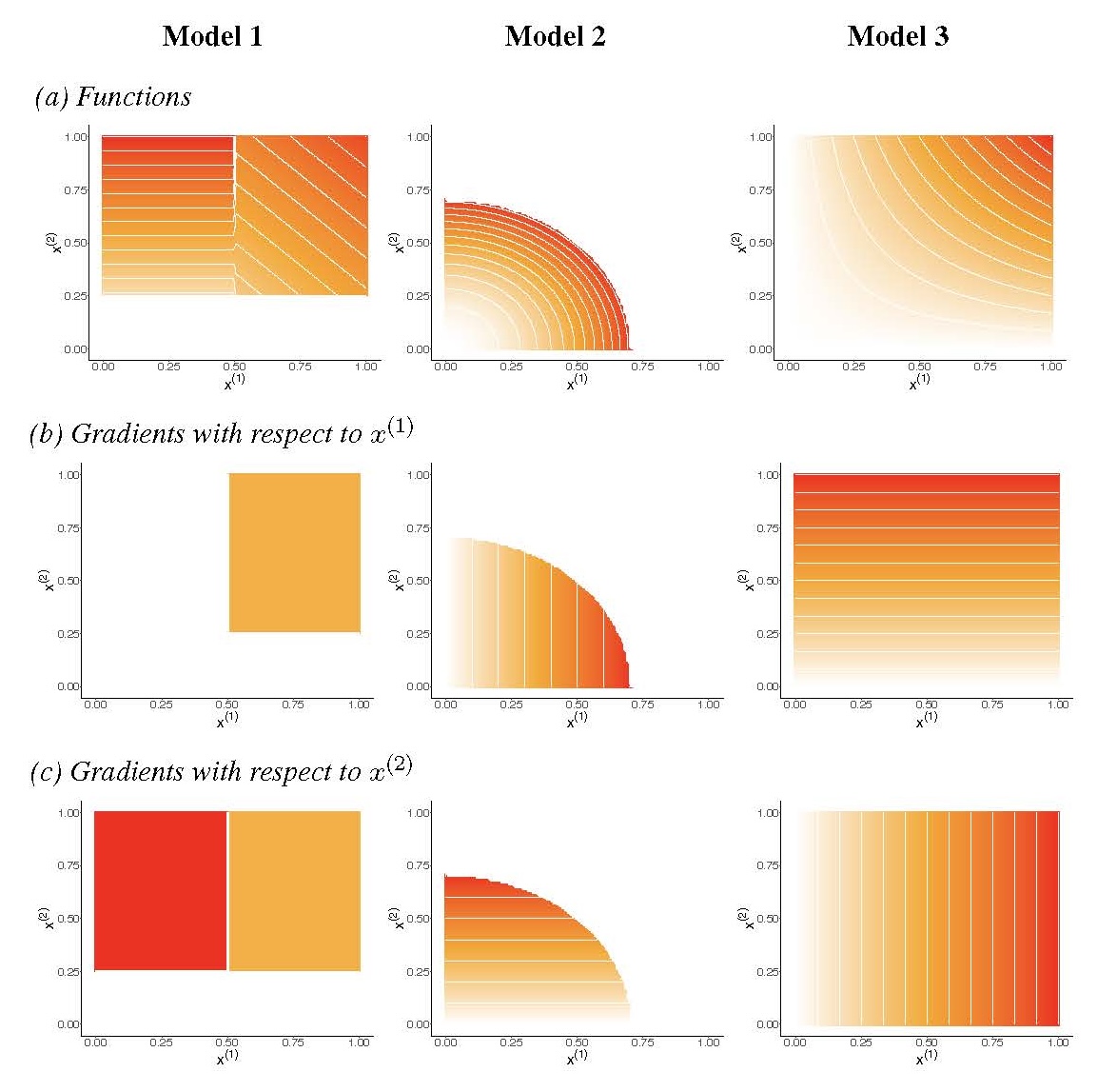
\[ \tiny{ \psi(x^{(1)}, x^{(2)}) = \begin{cases} 1, & x^{(2)} \leq 0.25, \\ 15x^{(2)}, & x^{(1)} \leq 0.5 \text{ and } x^{(2)} > 0.25, \\ 7x^{(1)} + 7x^{(2)}, & x^{(1)} > 0.5 \text{ and } x^{(2)} > 0.25 \end{cases} } \]

Model 2 is a quadratic function of the predictors, defining the response as a function of the squared Euclidean norm:

\[ \tiny{ \psi(x^{(1)}, x^{(2)}) = 5r 1_{\{r \leq 0.5\}}, \quad \text{where } r = (x^{(1)})^2 + (x^{(2)})^2 } \]

Model 3 follows a simple multiplicative interaction between the two predictors:

\[ \tiny{ \psi(x^{(1)}, x^{(2)}) = 6x^{(1)}x^{(2)} } \]

Simulation contour gradients

Comparison procedures

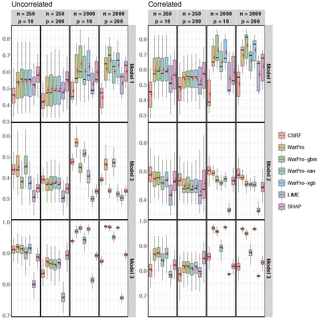
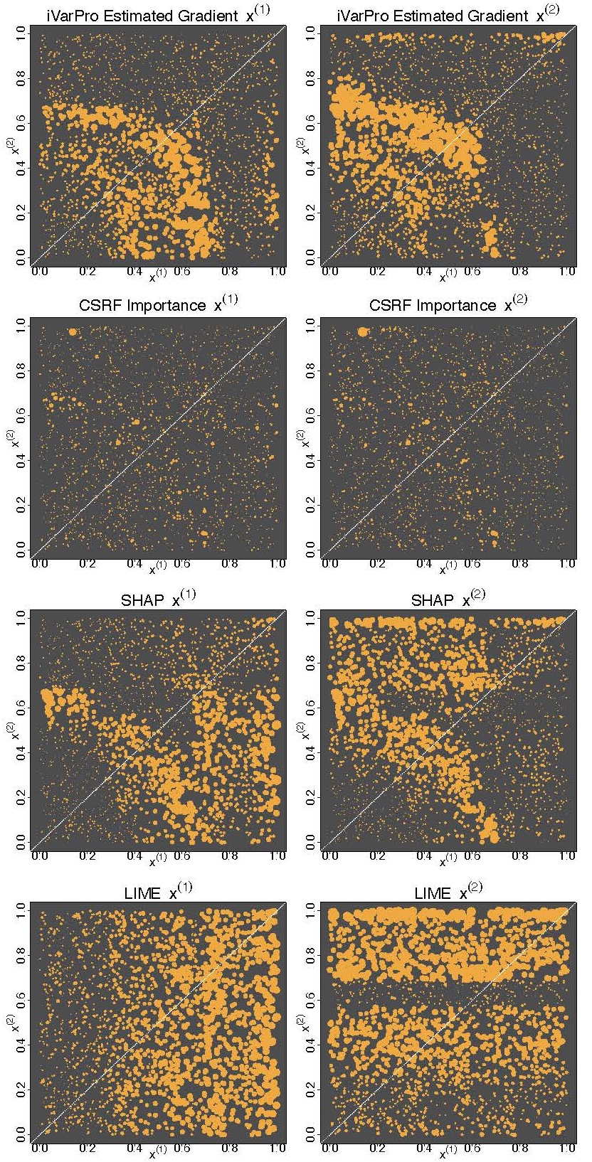
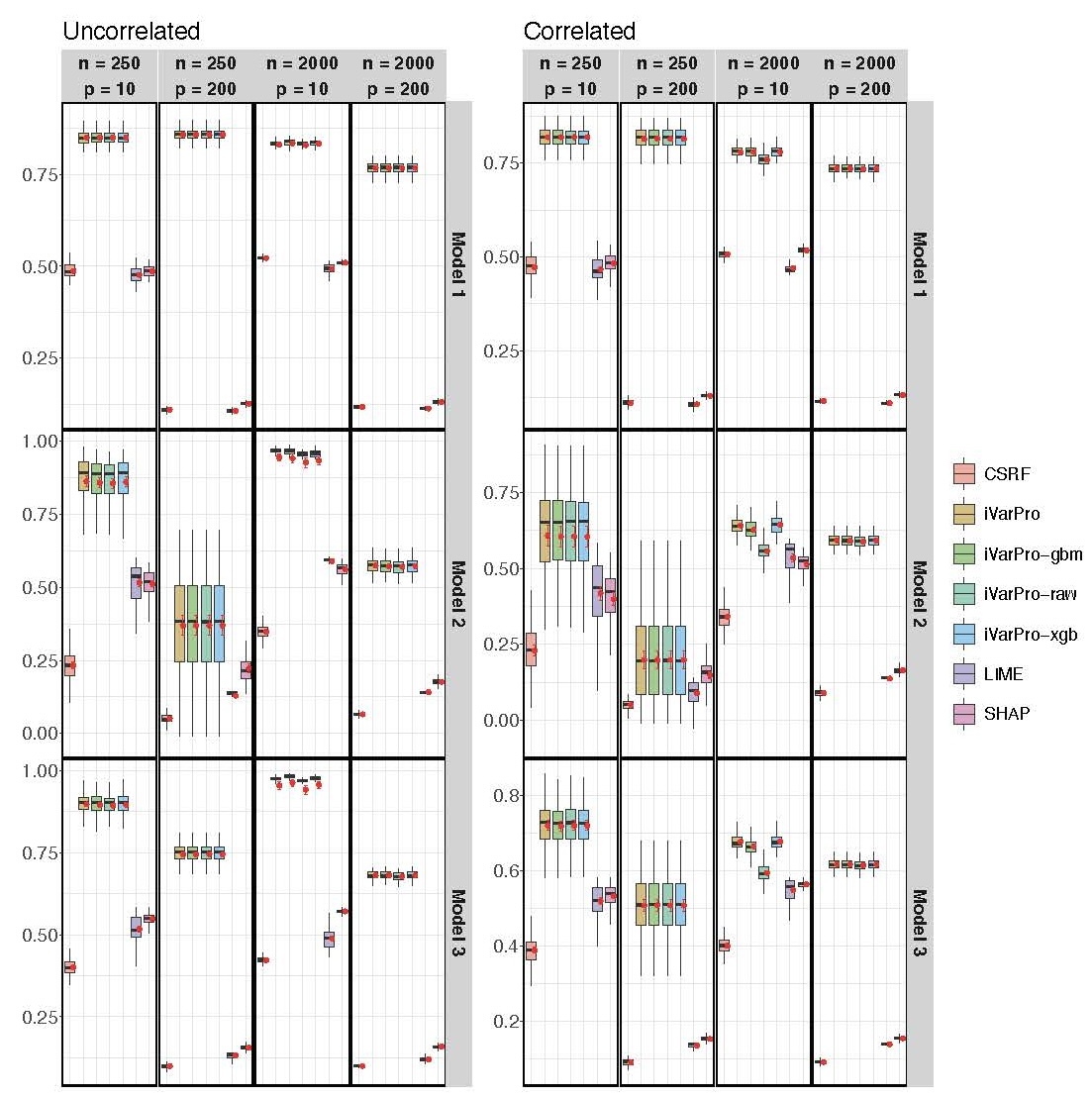
We compare iVarPro to three established methods:

CSRF (Case-Specific Random Forests) importance [2], implemented using the ranger R package [3]
SHAP, computed using the treeshap R package [4]
LIME, computed using the lime R package [5]

Both SHAP and LIME were applied to a trained XGBoost model [6], with hyperparameters selected via cross-validation. We also evaluate three additional versions of iVarPro based on different choices of the external predictor \({\widehat{\psi}}\):

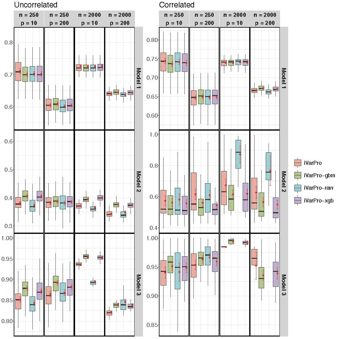
iVarPro-raw: No external model is used; local gradients are estimated directly using the raw response values \(y\)
iVarPro-gbm: The external predictor \({\widehat{\psi}}\) is a gradient tree boosted model fit using the gbm R package [7]
iVarPro-xgb: The external predictor \({\widehat{\psi}}\) is an XGBoost model

Simulation overview

Benchmark functions (piecewise, radial, interaction); \(p \in \{10,200\}\), \(n \in \{250,2000\}\)
Correlated/uncorrelated predictors: features for the uncorrelated setting are independently drawn from a Uniform\((0,1)\) distribution, and predictors for the correlated setting are drawn from a normal copula with common correlation \(\rho = 0.8\)
Compare iVarPro vs CSRF, SHAP, LIME
Metrics: Kendall’s \(\tau_b\), C-index, PR-AUC (ranking of true \(|\nabla\psi|\))

Simulation result

Kendall’s \(\tau_b\) scores evaluating the performance of iVarPro and comparison procedures in a synthetic setting. Red error bars denote 95% confidence intervals for the mean, slightly offset to the right for visual clarity

Uncorrelated gradient recovery

Simulation result

C-index scores evaluating the performance of iVarPro and comparison procedures in a synthetic setting

Uncorrelated gradient recovery

Simulation result

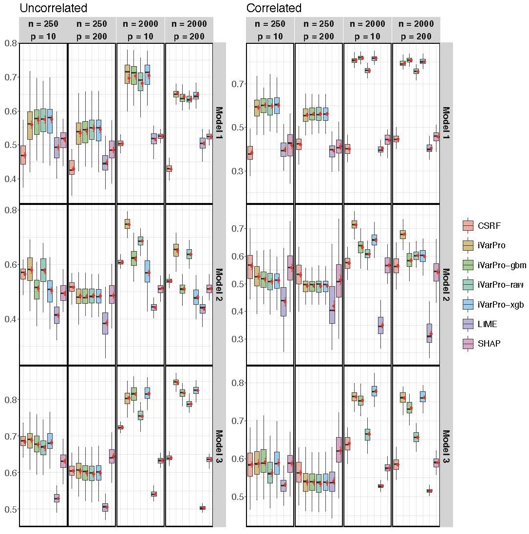
PR-AUC scores Uncorrelated gradient recovery

MSE scores Uncorrelated gradient recovery

A single run of Model 2 (uncorrelated)

Uncorrelated gradient recovery

A single run of Model 2 from iVarPro

Uncorrelated

Uncorrelated gradient recovery

Correlated

Uncorrelated gradient recovery

Synthetic survival example

The true (potentially unobserved) survival time:
\[ \def\Xs#1{X^{(#1)}} \def\x{{\bf x}} \def\X{{\bf X}} \def\PP{\mathbb{P}} \def\xs#1{x^{(#1)}} {\tiny T^o = \log \left[1 + V + \exp(\sum_{s=1}^4 \beta_s \Xs{s} + \beta_5 \Xs{5} 1_{\{\Xs{2} > 0.5\}} ) \right] } \] The variable \(\scriptsize V\) follows a standard exponential distribution and the features \(\scriptsize \Xs{s}\) is drawn from Uniform\(\scriptsize (0,1)\). We take \(\scriptsize \psi(\x)\) to be the restricted mean survival time (RMST) [11] up to a specified time horizon \(\scriptsize \tau>0\): \({\tiny \psi(\X) = \int_0^\tau S(t | \X)\,dt,}\) where \({\tiny S(t|\x) = \PP\{T^o > t | \X=\x\}}\)

To derive a closed-form expression for the gradient of \(\scriptsize \psi(\x)\), we have \({\tiny S(t|\x) =\PP\left\{ \log [1 + V + A(\x) ] > t \right\}},\) where \({\tiny A(\x) = \exp (\sum_{s=1}^4 \beta_s \xs{s}}\) \({\tiny+ \beta_5 \xs{5} 1_{\{\xs{2} > 0.5\}})}\)

We obtain the partial derivatives: \[ \def\L{\Lambda} {\tiny \begin{array} \frac{\partial \psi(\x)}{\partial \xs{s}} &=& \beta_s A(\x) e^{A(\x)} \L(\tau), \quad s = 1,2,3,4\\ \frac{\partial \psi(\x)}{\partial \xs{5}} &=& \beta_5 A(\x) e^{A(\x)} \L(\tau) 1_{\{\xs{2} > 0.5\}} \end{array} } \] Parameters were \(\beta_s = 2\) for \(s = 1, \ldots, 5\), and additionally, 15 noise variables were included, resulting in a total of \(p = 20\) features. Random censoring at a 25% rate was applied, and a total of \(n = 2000\) data points were sampled

Synthetic survival example

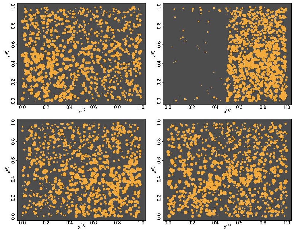
We obtain the partial derivatives: \[ \def\L{\Lambda} {\tiny \begin{array} \frac{\partial \psi(\x)}{\partial \xs{s}} &=& \beta_s A(\x) e^{A(\x)} \L(\tau), \quad s = 1,2,3,4\\ \frac{\partial \psi(\x)}{\partial \xs{5}} &=& \beta_5 A(\x) e^{A(\x)} \L(\tau) 1_{\{\xs{2} > 0.5\}} \end{array} } \] The figure below shows the estimated iVarPro values where \(\scriptsize \xs{5}\) has a smaller effect that is modulated by \(\scriptsize \xs{2}\) and influences survival only \(\scriptsize \xs{2} > 0.5\) Uncorrelated gradient recovery

Survival use case: CAD treadmill cohort

18,964 patients who underwent treadmill exercise testing for the evaluation of suspected coronary artery disease (CAD). Notably, all patients had a clinically normal resting electrocardiogram (ECG) and no known history of cardiovascular disease at the time of testing
outcome: all-cause mortality
\(\psi\): integrated cumulative hazard; \(\widehat{\psi}\): random survival forest

Results

Population leaders: Peak METs (Metabolic Equivalents at Peak Exercise), Duke Treadmill Score (DTS)
iVarPro finds ECG features with localized importance

ECG vs Clinical gradients

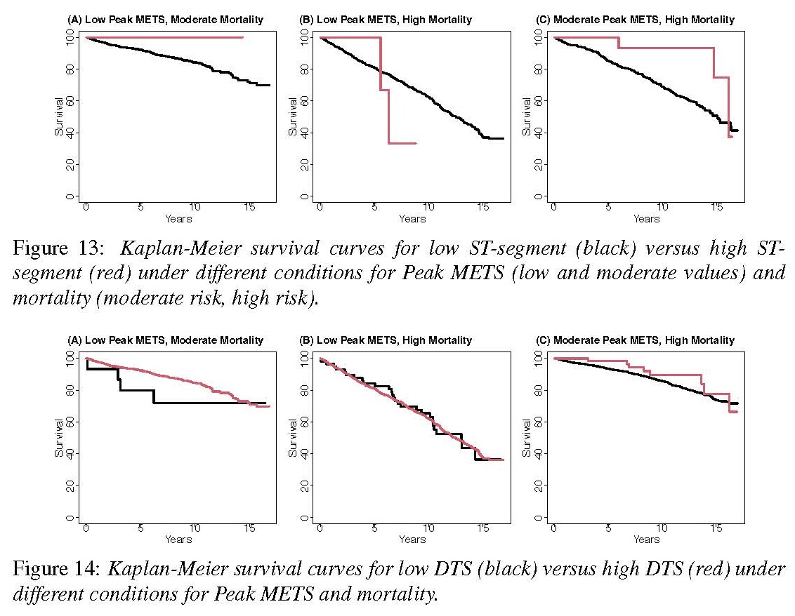
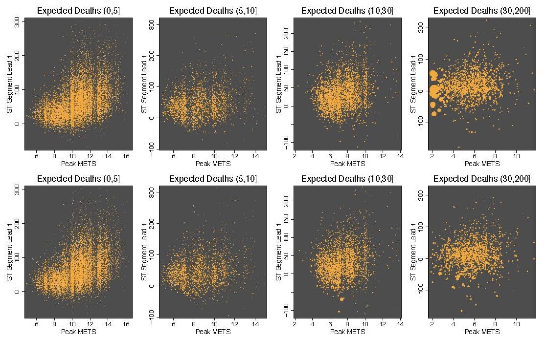
Visualizing clinical variable (Peak METs) versus ECG variable (ST-segment above the baseline)

The top panel scales circle size by the Peak METs gradient, and the bottom panel scales by the ECG gradient. Data are stratified by patient mortality

ECG vs survival gradients

Same as left, but with the vertical axis representing the Duke Treadmill Score (DTS). Circle are scaled to the gradients for Peak METs and DTS, respectively

ECG vs survival gradients

Kaplan–Meier sanity checks

Summary

iVarPro = local gradient importance using rules + release
Model-independent, data-grounded, individualized
Robust in high \(p\), correlated features; empirically strong vs SHAP/LIME/CSRF
Practical for precision medicine: surfaces what matters for this person

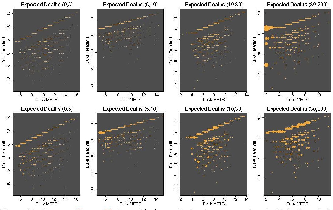
Message: population signals + patient-specific signals → better precision interpretation

Preprint: Lu M. and Ishwaran H. (2024). Model-independent variable selection via the rule-based variable priority.

Publication: Lu M. and Ishwaran H. (2025). Individual variable priority: A model-independent local gradient method for variable importance. To appear in Artifical Intelligence Review

Slides: https://luminwin.github.io/iVarPro

Presentation: https://youtu.be/wtUB9wkipwI

Looking ahead

Time-varying and longitudinal extensions
Causal framing for counterfactual gradients
Software: VarPro/iVarPro R packages and vignettes

Thanks!
Questions that change the gradient welcome!

References

1. Lu M, Ishwaran H. Model-independent variable selection via the rule-based variable priority. arXiv. 2024;2409.09003. https://arxiv.org/abs/2409.09003.

2. Xu R, Nettleton D, Nordman DJ. Case-specific random forests. Journal of Computational and Graphical Statistics. 2016;25:49–65.

3. Wright MN, Ziegler A. Ranger: A fast implementation of random forests for high dimensional data in C++ and R. Journal of Statistical Software. 2017;77:1–17. doi:10.18637/jss.v077.i01.

4. Komisarczyk K, Kozminski P, Maksymiuk S, Kapsner LA, Spytek M, Krzyzinski M, et al. Treeshap: Compute SHAP values for your tree-based models using the ’TreeSHAP’ algorithm. 2024. https://cran.r-project.org/package=treeshap.

5. Pedersen TL, Benesty M. Lime: Local interpretable model-agnostic explanations. 2022. https://cran.r-project.org/package=lime.

6. Chen T, Guestrin C. XGBoost: A scalable tree boosting system. Proceedings of the 22nd ACM SIGKDD International Conference on Knowledge Discovery and Data Mining (KDD ’16). 2016;785–94. doi:10.1145/2939672.2939785.

7. Greenwell B, Boehmke B, Cunningham J, Developers G. Gbm: Generalized boosted regression models. 2020. https://CRAN.R-project.org/package=gbm.

8. Irwin JO. The standard error of an estimate of expectation of life, with special reference to expectation of tumourless life in experiments with mice. Epidemiology & Infection. 1949;47:188–9.

9. Andersen PK, Hansen MG, Klein JP. Regression analysis of restricted mean survival time based on pseudo-observations. Lifetime Data Analysis. 2004;10:335–50.

10. Royston P, Parmar MKB. The use of restricted mean survival time to estimate the treatment effect in randomized clinical trials when the proportional hazards assumption is in doubt. Statistics in Medicine. 2011;30:2409–21.

11. Kim DH, Uno H, Wei L-J. Restricted mean survival time as a measure to interpret clinical trial results. JAMA Cardiology. 2017;2:1179–80.