| PID | MS.SubClass | MS.Zoning | Lot.Frontage | Lot.Area | Street | Alley | Lot.Shape | Land.Contour | Utilities | Lot.Config | Land.Slope | Neighborhood | Condition.1 | Condition.2 | Bldg.Type | House.Style | Overall.Qual | Overall.Cond | Year.Built | Year.Remod.Add | Roof.Style | Roof.Matl | Exterior.1st | Exterior.2nd | Mas.Vnr.Type | Mas.Vnr.Area | Exter.Qual | Exter.Cond | Foundation | Bsmt.Qual | Bsmt.Cond | Bsmt.Exposure | BsmtFin.Type.1 | BsmtFin.SF.1 | BsmtFin.Type.2 | BsmtFin.SF.2 | Bsmt.Unf.SF | Total.Bsmt.SF | Heating | Heating.QC | Central.Air | Electrical | X1st.Flr.SF | X2nd.Flr.SF | Low.Qual.Fin.SF | Gr.Liv.Area | Bsmt.Full.Bath | Bsmt.Half.Bath | Full.Bath | Half.Bath | Bedroom.AbvGr | Kitchen.AbvGr | Kitchen.Qual | TotRms.AbvGrd | Functional | Fireplaces | Fireplace.Qu | Garage.Type | Garage.Yr.Blt | Garage.Finish | Garage.Cars | Garage.Area | Garage.Qual | Garage.Cond | Paved.Drive | Wood.Deck.SF | Open.Porch.SF | Enclosed.Porch | X3Ssn.Porch | Screen.Porch | Pool.Area | Pool.QC | Fence | Misc.Feature | Misc.Val | Mo.Sold | Yr.Sold | Sale.Type | Sale.Condition | SalePrice |
|---|---|---|---|---|---|---|---|---|---|---|---|---|---|---|---|---|---|---|---|---|---|---|---|---|---|---|---|---|---|---|---|---|---|---|---|---|---|---|---|---|---|---|---|---|---|---|---|---|---|---|---|---|---|---|---|---|---|---|---|---|---|---|---|---|---|---|---|---|---|---|---|---|---|---|---|---|---|---|---|---|
| 526301100 | 20 | RL | 141 | 31770 | Pave | noAlleyAccess | IR1 | Lvl | AllPub | Corner | Gtl | NAmes | Norm | Norm | 1Fam | 1Story | 6 | 5 | 1960 | 1960 | Hip | CompShg | BrkFace | Plywood | Stone | 112 | TA | TA | CBlock | TA | Gd | Gd | BLQ | 639 | Unf | 0 | 441 | 1080 | GasA | Fa | Y | SBrkr | 1656 | 0 | 0 | 1656 | 1 | 0 | 1 | 0 | 3 | 1 | TA | 7 | Typ | 2 | Gd | Attchd | 1960 | Fin | 2 | 528 | TA | TA | P | 210 | 62 | 0 | 0 | 0 | 0 | noPool | noFence | none | 0 | 5 | 2010 | WD | Normal | 215000 |
| 526350040 | 20 | RH | 80 | 11622 | Pave | noAlleyAccess | Reg | Lvl | AllPub | Inside | Gtl | NAmes | Feedr | Norm | 1Fam | 1Story | 5 | 6 | 1961 | 1961 | Gable | CompShg | VinylSd | VinylSd | None | 0 | TA | TA | CBlock | TA | TA | No | Rec | 468 | LwQ | 144 | 270 | 882 | GasA | TA | Y | SBrkr | 896 | 0 | 0 | 896 | 0 | 0 | 1 | 0 | 2 | 1 | TA | 5 | Typ | 0 | noFireplace | Attchd | 1961 | Unf | 1 | 730 | TA | TA | Y | 140 | 0 | 0 | 0 | 120 | 0 | noPool | MnPrv | none | 0 | 6 | 2010 | WD | Normal | 105000 |
| 526351010 | 20 | RL | 81 | 14267 | Pave | noAlleyAccess | IR1 | Lvl | AllPub | Corner | Gtl | NAmes | Norm | Norm | 1Fam | 1Story | 6 | 6 | 1958 | 1958 | Hip | CompShg | Wd Sdng | Wd Sdng | BrkFace | 108 | TA | TA | CBlock | TA | TA | No | ALQ | 923 | Unf | 0 | 406 | 1329 | GasA | TA | Y | SBrkr | 1329 | 0 | 0 | 1329 | 0 | 0 | 1 | 1 | 3 | 1 | Gd | 6 | Typ | 0 | noFireplace | Attchd | 1958 | Unf | 1 | 312 | TA | TA | Y | 393 | 36 | 0 | 0 | 0 | 0 | noPool | noFence | Gar2 | 12500 | 6 | 2010 | WD | Normal | 172000 |
| 526353030 | 20 | RL | 93 | 11160 | Pave | noAlleyAccess | Reg | Lvl | AllPub | Corner | Gtl | NAmes | Norm | Norm | 1Fam | 1Story | 7 | 5 | 1968 | 1968 | Hip | CompShg | BrkFace | BrkFace | None | 0 | Gd | TA | CBlock | TA | TA | No | ALQ | 1065 | Unf | 0 | 1045 | 2110 | GasA | Ex | Y | SBrkr | 2110 | 0 | 0 | 2110 | 1 | 0 | 2 | 1 | 3 | 1 | Ex | 8 | Typ | 2 | TA | Attchd | 1968 | Fin | 2 | 522 | TA | TA | Y | 0 | 0 | 0 | 0 | 0 | 0 | noPool | noFence | none | 0 | 4 | 2010 | WD | Normal | 244000 |
| 527105010 | 60 | RL | 74 | 13830 | Pave | noAlleyAccess | IR1 | Lvl | AllPub | Inside | Gtl | Gilbert | Norm | Norm | 1Fam | 2Story | 5 | 5 | 1997 | 1998 | Gable | CompShg | VinylSd | VinylSd | None | 0 | TA | TA | PConc | Gd | TA | No | GLQ | 791 | Unf | 0 | 137 | 928 | GasA | Gd | Y | SBrkr | 928 | 701 | 0 | 1629 | 0 | 0 | 2 | 1 | 3 | 1 | TA | 6 | Typ | 1 | TA | Attchd | 1997 | Fin | 2 | 482 | TA | TA | Y | 212 | 34 | 0 | 0 | 0 | 0 | noPool | MnPrv | none | 0 | 3 | 2010 | WD | Normal | 189900 |
| 527105030 | 60 | RL | 78 | 9978 | Pave | noAlleyAccess | IR1 | Lvl | AllPub | Inside | Gtl | Gilbert | Norm | Norm | 1Fam | 2Story | 6 | 6 | 1998 | 1998 | Gable | CompShg | VinylSd | VinylSd | BrkFace | 20 | TA | TA | PConc | TA | TA | No | GLQ | 602 | Unf | 0 | 324 | 926 | GasA | Ex | Y | SBrkr | 926 | 678 | 0 | 1604 | 0 | 0 | 2 | 1 | 3 | 1 | Gd | 7 | Typ | 1 | Gd | Attchd | 1998 | Fin | 2 | 470 | TA | TA | Y | 360 | 36 | 0 | 0 | 0 | 0 | noPool | noFence | none | 0 | 6 | 2010 | WD | Normal | 195500 |
Tree-Based Machine Learning Methods for Prediction and Variable Selection
Part I
Hemant Ishwaran and Min Lu
University of Miami
University of Miami
Brief Overview
This cover covers the following R packages
-
randomForestSRC: Fast Unified Random Forests for Survival, Regression, and Classification (CRAN link) -
randomForestSRC.run: Integrated visualization for therandomForestSRCpackage (Github link) -
varPro: Model-Independent Variable Selection via the Rule-Based Variable Priority (Github link)
Outline
Part I: Training
- Brief overview
- Quick start
- Training (grow) with examples
(regression, classification, survival)
Part II: Inference and Prediction
- Inference (OOB)
- Prediction Error
- Prediction
- Restore
- Partial Plots
Part III: Variable Selection
- VIMP
- Subsampling (Confidence Intervals)
- Minimal Depth
- VarPro
Part IV: Advanced Examples
- Class Imbalanced Data
- Competing Risks
- Multivariate Forests
- Missing data imputation
Brief Overview
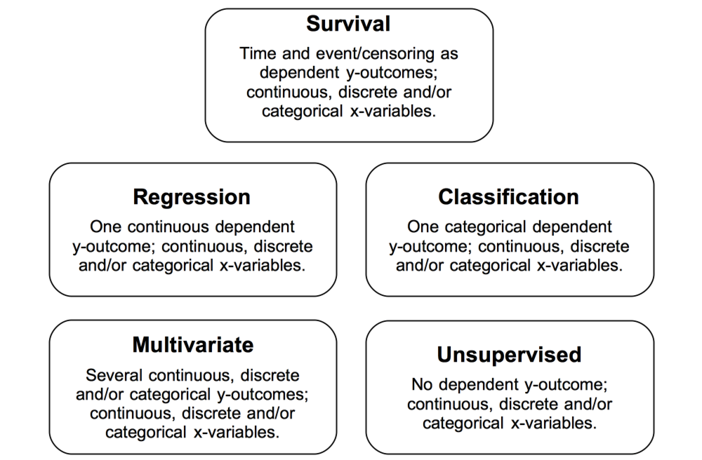
randomForestSRC is a fast OpenMP and memory efficient package for fitting random forests (RF) for univariate, multivariate, unsupervised, survival, competing risks, class imbalanced classification and quantile regression
Brief Overview
A random forest (RF) [1] consists of a collection of random tree structured predictors {\(h({\bf x},{{\bf\Theta}_b}), b= 1,2,\ldots, B\)} where {\({{\bf\Theta}_b}\)} are independent identically distributed random vectors. The RF predictor is the ensemble \[F_{{\!\text{ens}}}({\bf x})=\frac{1}{B}\sum_{b=1}^B h({\bf x},{{\bf\Theta}_b})\]
Typically, \({{\bf\Theta}_b}\) encode the instructions for bootstrapping the data and for random feature selection used for tree splitting
Brief Overview
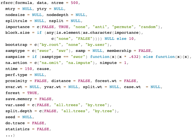
rfsrc(formula, data, ntree, mtry, nodesize)
| Family | Example Grow Call with Formula Specification |
|---|---|
| Survival | rfsrc(Surv(time, status)~., data = veteran) |
| Competing Risk | rfsrc(Surv(time, status)~., data = wihs) |
| Regression Quantile Regression |
rfsrc(Ozone~., data = airquality) quantreg(mpg~., data = mtcars)
|
| Classification Imbalanced Two-Class |
rfsrc(Species~., data = iris) imbalanced(status~., data = breast)
|
| Multivariate Regression Multivariate Mixed Regression Multivariate Quantile Regression Multivariate Mixed Quantile Regression |
rfsrc(Multivar(mpg, cyl)~., data = mtcars) rfsrc(cbind(Species,Sepal.Length)~.,data=iris) quantreg(cbind(mpg, cyl)~., data = mtcars) quantreg(cbind(Species,Sepal.Length)~.,data=iris)
|
| Unsupervised sidClustering Breiman (Shi-Horvath) |
rfsrc(data = mtcars) sidClustering(data = mtcars) sidClustering(data = mtcars, method = "sh")
|
Learn more [2]: https://www.randomforestsrc.org/articles/getstarted.html
Quick Start: Iowa Housing
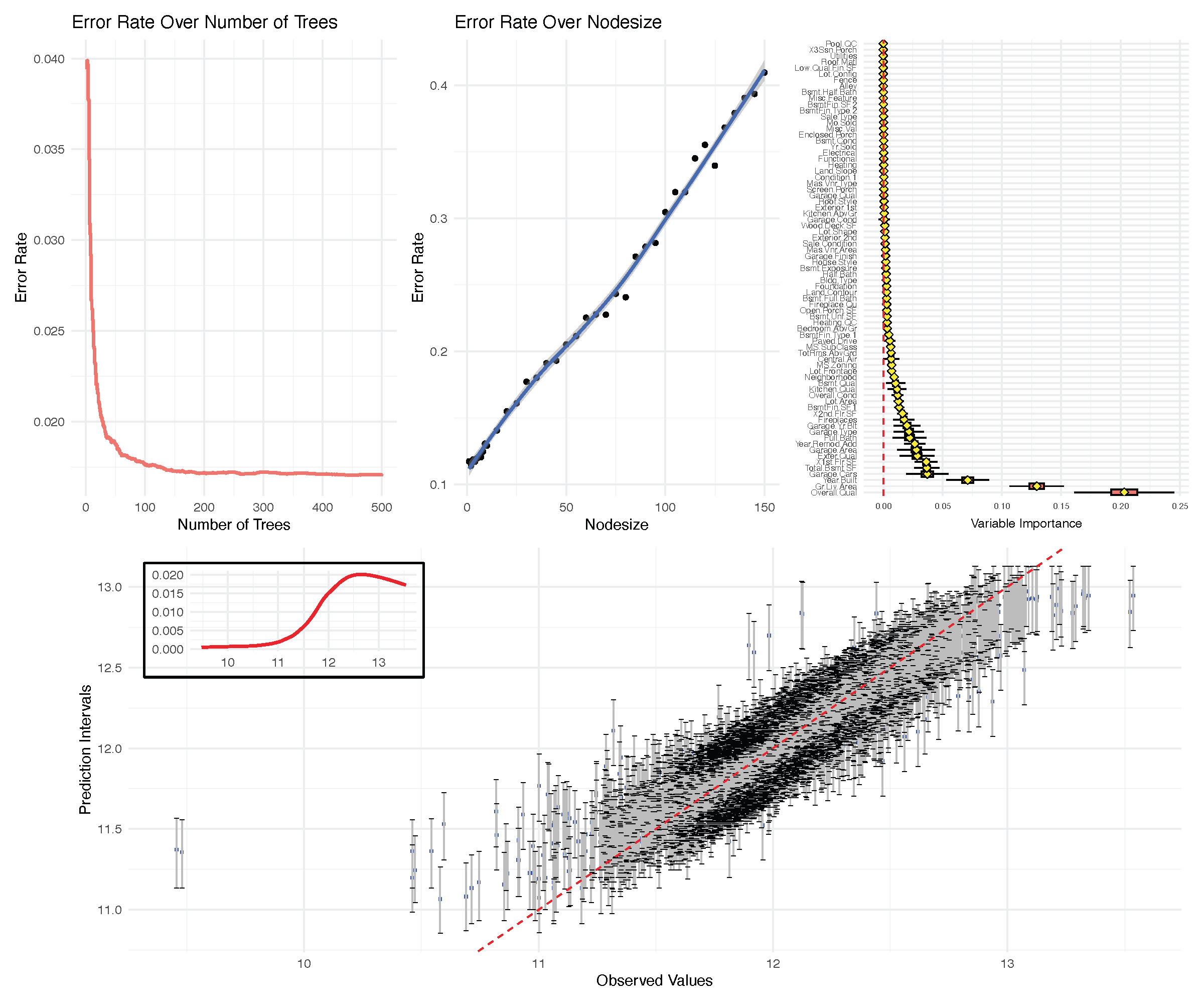
Ames Iowa Housing Data
Data from the Ames Assessor’s Office used in assessing values of individual residential properties sold in Ames, Iowa from 2006 to 2010. This is a regression problem and the goal is to predict “SalePrice” which records the price of a home in thousands of dollars [3]
Quick Start
flowchart LR
  A[Grow a forest] --> B[Check the output] --> C[Make the prediction]
Quick Start
flowchart LR
  A[<h3 style="color:darkgreen">Grow a forest</h3>] --> B[Check the output] --> C[Make the prediction]
Quick Start
flowchart LR A[Grow a forest] --> B[<h3 style="color:darkgreen">Check the output</h3>] --> C[Make the prediction]
library(randomForestSRC)
o <- rfsrc(SalePrice~., data = housing)
print(o)
> 1 Sample size: 2274
> 2 Number of trees: 500
> 3 Forest terminal node size: 5
> 4 Average no. of terminal nodes: 311.04
> 5 No. of variables tried at each split: 27
> 6 Total no. of variables: 80
> 7 Resampling used to grow trees: swor
> 8 Resample size used to grow trees: 1437
> 9 Analysis: RF-R
> 10 Family: regr
> 11 Splitting rule: mse *random*
> 12 Number of random split points: 10
>  13                      (OOB) R squared: 0.90947926
> 14 (OOB) Requested performance error: 628691481.703799Quick Start
Tip
The last line(s) will show the cross validated prediction performance
- Model performance is displayed in the last two lines in terms of out-of-bag (OOB) prediction error. In regression, this the cross-validated (leave-one-out bootstrap) mean squared error (MSE) estimated via the out-of-bag data shown in line 14
- Since MSE is scale dependent, standardized MSE, defined as the MSE divided by the variance of the outcome, is used and converted to R squared (or percent variance explained) which has an intuitive and universal interpretation, shown in line 13
Quick Start: Iowa Housing
Transform the outcome
Tip
Monotonic transformation on the outcome won’t substantially change the structure of random forest due to its robustness. However, it may be useful for scaling the mean squared error
o <- rfsrc(SalePrice~., data= housing)
o
>  1                           Sample size: 2274
>  2                       Number of trees: 500
>  3             Forest terminal node size: 5
>  4         Average no. of terminal nodes: 311.04
>  5  No. of variables tried at each split: 27
>  6                Total no. of variables: 80
>  7         Resampling used to grow trees: swor
>  8      Resample size used to grow trees: 1437
>  9                              Analysis: RF-R
>  10                               Family: regr
>  11                       Splitting rule: mse *random*
>  12        Number of random split points: 10
>  13                      (OOB) R squared: 0.90947926
>  14    (OOB) Requested performance error: 628691481.703799
> housing$SalePrice <- log(housing$SalePrice)
> o <- rfsrc(SalePrice~., data= housing)
> o
> 1 Sample size: 2274
> 2 Number of trees: 500
> 3 Forest terminal node size: 5
> 4 Average no. of terminal nodes: 310.61
> 5 No. of variables tried at each split: 27
> 6 Total no. of variables: 80
> 7 Resampling used to grow trees: swor
> 8 Resample size used to grow trees: 1437
> 9 Analysis: RF-R
> 10 Family: regr
> 11 Splitting rule: mse *random*
> 12 Number of random split points: 10
> 13 (OOB) R squared: 0.89837879
> 14 (OOB) Requested performance error: 0.01688687Quick Start
Terminal Output
data(housing, package = "randomForestSRC")
housing$SalePrice <- log(housing$SalePrice)
o <- rfsrc(SalePrice~., data= housing)
print(o)


>  1                           Sample size: 2274
>  2                       Number of trees: 500
>  3             Forest terminal node size: 5
>  4         Average no. of terminal nodes: 310.61
>  5  No. of variables tried at each split: 27
>  6                Total no. of variables: 80
>  7         Resampling used to grow trees: swor
>  8      Resample size used to grow trees: 1437
>  9                              Analysis: RF-R
>  10                               Family: regr
>  11                       Splitting rule: mse *random*
>  12        Number of random split points: 10
>  13                      (OOB) R squared: 0.89837879
> 14 (OOB) Requested performance error: 0.01688687Default is number of variables divided by 3 for regression. For all other families (including unsupervised settings), it is the square root of number of variables. Values are rounded up
Quick Start
Terminal Output
data(housing, package = "randomForestSRC")
housing$SalePrice <- log(housing$SalePrice)
o <- rfsrc(SalePrice~., data= housing)
print(o)


>  1                           Sample size: 2274
>  2                       Number of trees: 500
>  3             Forest terminal node size: 5
>  4         Average no. of terminal nodes: 310.61
>  5  No. of variables tried at each split: 27
>  6                Total no. of variables: 80
>  7         Resampling used to grow trees: swor
>  8      Resample size used to grow trees: 1437
>  9                              Analysis: RF-R
>  10                               Family: regr
>  11                       Splitting rule: mse *random*
>  12        Number of random split points: 10
>  13                      (OOB) R squared: 0.89837879
> 14 (OOB) Requested performance error: 0.01688687line 8 displays the sample size for line 7 where for swor, the number equals to about 63.2% observations, which matches the usual bootstrap sample size
Quick Start
Terminal Output
data(housing, package = "randomForestSRC")
housing$SalePrice <- log(housing$SalePrice)
o <- rfsrc(SalePrice~., data= housing)
print(o)


>  1                           Sample size: 2274
>  2                       Number of trees: 500
>  3             Forest terminal node size: 5
>  4         Average no. of terminal nodes: 310.61
>  5  No. of variables tried at each split: 27
>  6                Total no. of variables: 80
>  7         Resampling used to grow trees: swor
>  8      Resample size used to grow trees: 1437
>  9                              Analysis: RF-R
>  10                               Family: regr
>  11                       Splitting rule: mse *random*
>  12        Number of random split points: 10
>  13                      (OOB) R squared: 0.89837879
>  14    (OOB) Requested performance error: 0.01688687
Explanation
line 9 and 10 show the type of forest where RF-R and regr refer to regression
Quick Start
Terminal Output
data(housing, package = "randomForestSRC")
housing$SalePrice <- log(housing$SalePrice)
o <- rfsrc(SalePrice~., data= housing)
print(o)


>  1                           Sample size: 2274
>  2                       Number of trees: 500
>  3             Forest terminal node size: 5
>  4         Average no. of terminal nodes: 310.61
>  5  No. of variables tried at each split: 27
>  6                Total no. of variables: 80
>  7         Resampling used to grow trees: swor
>  8      Resample size used to grow trees: 1437
>  9                              Analysis: RF-R
>  10                               Family: regr
>  11                       Splitting rule: mse *random*
>  12        Number of random split points: 10
>  13                      (OOB) R squared: 0.89837879
> 14 (OOB) Requested performance error: 0.01688687Quick Start
Terminal Output
data(housing, package = "randomForestSRC")
housing$SalePrice <- log(housing$SalePrice)
o <- rfsrc(SalePrice~., data= housing)
print(o)


>  1                           Sample size: 2274
>  2                       Number of trees: 500
>  3             Forest terminal node size: 5
>  4         Average no. of terminal nodes: 310.61
>  5  No. of variables tried at each split: 27
>  6                Total no. of variables: 80
>  7         Resampling used to grow trees: swor
>  8      Resample size used to grow trees: 1437
>  9                              Analysis: RF-R
>  10                               Family: regr
>  11                       Splitting rule: mse *random*
>  12        Number of random split points: 10
>  13                      (OOB) R squared: 0.89837879
> 14 (OOB) Requested performance error: 0.01688687Quick Start
flowchart LR
  A[Grow a forest] --> B[Check the output] --> C[<h3 style="color:darkgreen">Make the prediction</h3>]
General call to rfsrc
General call to rfsrc.cart
rfsrc.cart(formula, data, ntree = 1, mtry = ncol(data), bootstrap = “none”, …)
Tip: convenient interface for growing a Classification And Regression Tree (CART)
rfsrc.cart() is useful for growing single trees of almost any type
Nonparametric regression
| Family | Example Grow Call with Formula Specification |
|---|---|
|
Regression Quantile Regression |
rfsrc(Ozone~., data = airquality) quantreg(mpg~., data = mtcars) |
| Classification Imbalanced Two-Class |
rfsrc(Species~., data = iris) imbalanced(status~., data = breast)
|
| Survival | rfsrc(Surv(time, status)~., data = veteran) |
| Competing Risk | rfsrc(Surv(time, status)~., data = wihs) |
| Multivariate Regression Multivariate Mixed Regression Multivariate Quantile Regression Multivariate Mixed Quantile Regression |
rfsrc(Multivar(mpg, cyl)~., data = mtcars) rfsrc(cbind(Species,Sepal.Length)~.,data=iris) quantreg(cbind(mpg, cyl)~., data = mtcars) quantreg(cbind(Species,Sepal.Length)~.,data=iris)
|
| Unsupervised sidClustering Breiman (Shi-Horvath) |
rfsrc(data = mtcars) sidClustering(data = mtcars) sidClustering(data = mtcars, method = "sh")
|
Quantile Regression:
randomForestSRC vs Meinshausen
Meinshausen
Splitting rule: MSE
Conditional CDF: Terminal node CDF
randomForestSRC quantreg
Splitting rule: Pinball loss
splitrule = "la.quant.reg"Conditional CDF: Local estimator
method = "local"
Regression example: Iowa housing
Quantile regression
o <- quantreg(SalePrice ~ ., housing, splitrule = "mse", ntree = 250)
o <- quantreg(SalePrice ~ ., housing, splitrule = "quantile.regr", ntree = 250)
o <- quantreg(SalePrice ~ ., housing, splitrule = "la.quantile.regr", ntree = 250) # (default)
> o
Sample size: 2274
Number of trees: 250
Forest terminal node size: 5
Average no. of terminal nodes: 263.86
No. of variables tried at each split: 27
Total no. of variables: 80
Resampling used to grow trees: swor
Resample size used to grow trees: 1437
Analysis: RF-R
Family: regr
Splitting rule: la.quantile.regr *random*
Number of random split points: 10
(OOB) R squared: 0.85752024
(OOB) Requested performance error: 0.02367652
Regression example: Iowa housing
The run.rfsrc function for an overview
Runs rfsrc on a user’s specified data and performs a detailed analysis including tuning the forests and plotting various quantities such as performance metrics and variable importance. Applies to regression, classification, survival, competing risk and multivariate families
Regression example: Iowa housing
Classification
| Family | Example Grow Call with Formula Specification |
|---|---|
|
Regression Quantile Regression |
rfsrc(Ozone~., data = airquality) quantreg(mpg~., data = mtcars)
|
|
Classification Imbalanced Two-Class |
rfsrc(Species~., data = iris) imbalanced(status~., data = breast)
|
| Survival | rfsrc(Surv(time, status)~., data = veteran) |
| Competing Risk | rfsrc(Surv(time, status)~., data = wihs) |
| Multivariate Regression Multivariate Mixed Regression Multivariate Quantile Regression Multivariate Mixed Quantile Regression |
rfsrc(Multivar(mpg, cyl)~., data = mtcars) rfsrc(cbind(Species,Sepal.Length)~.,data=iris) quantreg(cbind(mpg, cyl)~., data = mtcars) quantreg(cbind(Species,Sepal.Length)~.,data=iris)
|
| Unsupervised sidClustering Breiman (Shi-Horvath) |
rfsrc(data = mtcars) sidClustering(data = mtcars) sidClustering(data = mtcars, method = "sh")
|
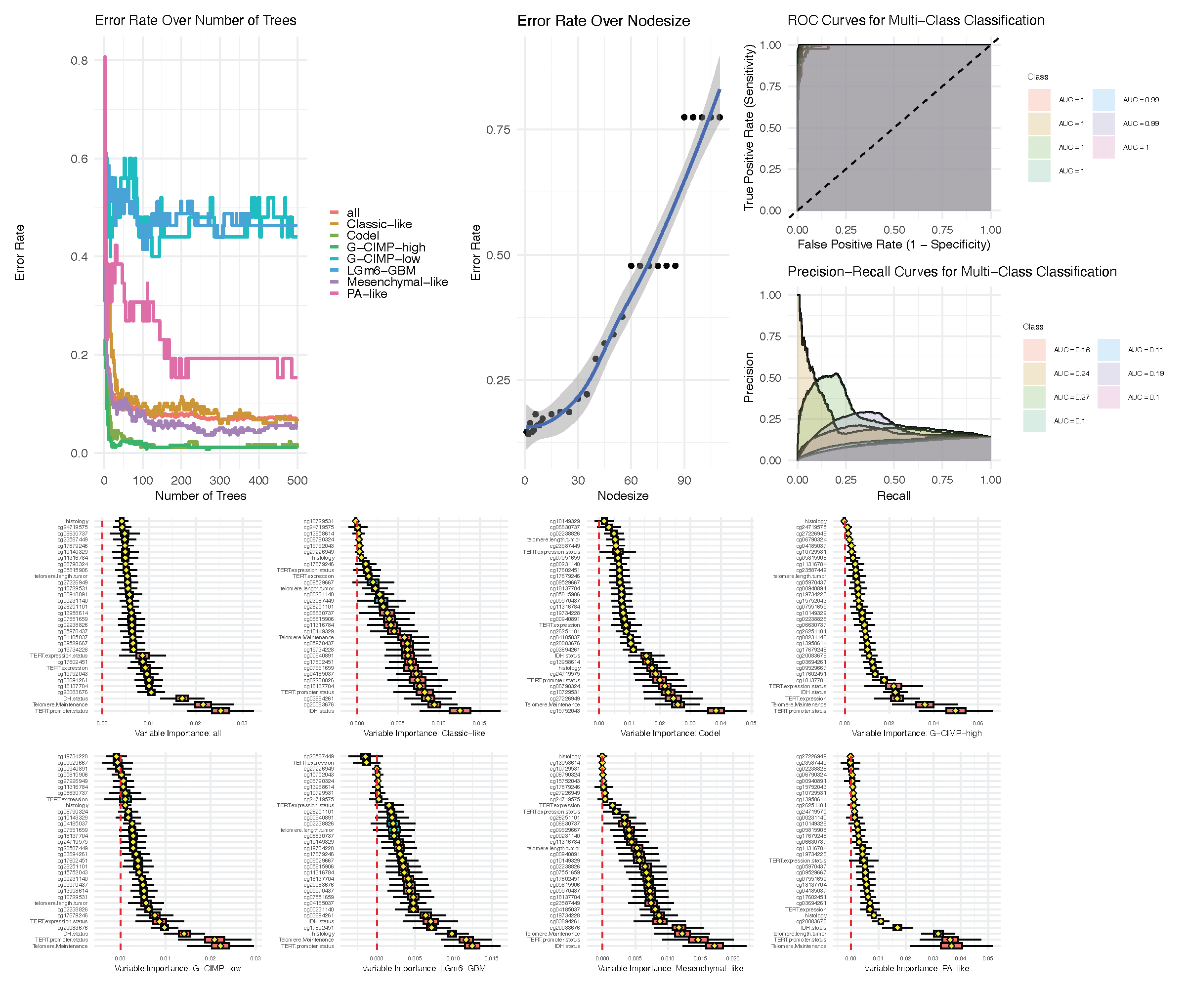
Classification example: Glioma
Subset of the data used in Ceccarelli et al. (2016) for molecular profiling of adult diffuse gliomas. It contains 1206 probes from 880 tissues, clinical data and other molecular data. The outcome has class labels: Classic-like, Codel, G-CIMP-high, G-CIMP-low, LGm6-GBM, Mesenchymal-like and PA-like [4]
| y | cg23970089 | cg25176823 | cg24576735 | Chr19.20co.gain | TERT.promoter.status | SNP6 | U133a | grade | age | gender |
|---|---|---|---|---|---|---|---|---|---|---|
| Mesenchymal-like | 0.36518600 | 0.3244530 | 0.03255164 | No chr 19/20 gain | Mutant | Yes | Yes | G4 | 44 | female |
| Mesenchymal-like | 0.60246131 | 0.3626941 | 0.02215452 | No chr 19/20 gain | Mutant | Yes | Yes | G4 | 50 | male |
| Mesenchymal-like | 0.44011951 | 0.3679728 | 0.03369096 | No chr 19/20 gain | Mutant | Yes | No | G4 | 56 | female |
| Classic-like | 0.06834791 | 0.3974054 | 0.03623296 | No chr 19/20 gain | Mutant | Yes | Yes | G4 | 40 | female |
| Classic-like | 0.19843219 | 0.2736760 | 0.04060163 | No chr 19/20 gain | Mutant | Yes | Yes | G4 | 61 | female |
Classification example: Glioma
o <- rfsrc(y~., data = glioma)
o
                         Sample size: 878
           Frequency of class labels: Classic-like=148, Codel=174, G-CIMP-high=249, G-CIMP-low=25, LGm6-GBM=41, Mesenchymal-like=215, PA-like=26
                     Number of trees: 500
           Forest terminal node size: 1
       Average no. of terminal nodes: 73.896
No. of variables tried at each split: 36
              Total no. of variables: 1241
       Resampling used to grow trees: swor
    Resample size used to grow trees: 555
                            Analysis: RF-C
                              Family: class
                      Splitting rule: gini *random*
       Number of random split points: 10
                   (OOB) Brier score: 0.02292715
        (OOB) Normalized Brier score: 0.18723839
                           (OOB) AUC: 0.99338879
                      (OOB) Log-loss: 0.33872539
   (OOB) Requested performance error: 0.07061503, 0.05405405, 0.01149425, 0.00803213, 0.52, 0.51219512, 0.06046512, 0.11538462

Confusion matrix:

                  predicted
  observed         Classic-like Codel G-CIMP-high G-CIMP-low LGm6-GBM Mesenchymal-like PA-like class.error
  Classic-like              140     0           0          0        0                8       0      0.0541
  Codel                       0   172           2          0        0                0       0      0.0115
  G-CIMP-high                 0     2         247          0        0                0       0      0.0080
  G-CIMP-low                  0     0          13         12        0                0       0      0.5200
  LGm6-GBM                    0     1           0          0       20               20       0      0.5122
  Mesenchymal-like           13     0           0          0        0              202       0      0.0605
  PA-like                     0     0           0          0        0                3      23      0.1154

      (OOB) Misclassification rate: 0.07061503

Random-classifier baselines (uniform):
   Brier: 0.12244898   Normalized Brier: 1   Log-loss: 1.94591015
Tip
rfsrc recognize classification problem automatically when the outcome is a factor
Classification example: Glioma
Split rules
| Family | splitrule |
|---|---|
| Regression Quantile Regression |
mse la.quantile.regr, quantile.regr, mse
|
|
Classification Imbalanced Two-Class |
gini, auc, entropy gini, auc, entropy
|
| Survival | logrank, bs.gradient, logrankscore |
| Competing Risk | logrankCR, logrank |
| Multivariate Regression Multivariate Classification Multivariate Mixed Regression Multivariate Quantile Regression Multivariate Mixed Quantile Regression |
mv.mse, mahalanobis mv.gini mv.mix mv.mse mv.mix
|
| Unsupervised sidClustering Breiman (Shi-Horvath) |
unsupv \(\{\) mv.mse, mv.gini, mv.mix\(\}\), mahalanobis gini, auc, entropy
|
Learn more [5]: https://www.randomforestsrc.org/articles/aucsplit.html
Classification example: Glioma
Split rules: Gini index splitting (default)
o <- rfsrc(y~., data = glioma,
           splitrule="gini") ## default splitrule as in the previous slide
o
                         Sample size: 878
           Frequency of class labels: Classic-like=148, Codel=174, G-CIMP-high=249, G-CIMP-low=25, LGm6-GBM=41, Mesenchymal-like=215, PA-like=26
                     Number of trees: 500
           Forest terminal node size: 1
       Average no. of terminal nodes: 73.636
No. of variables tried at each split: 36
              Total no. of variables: 1241
       Resampling used to grow trees: swor
    Resample size used to grow trees: 555
                            Analysis: RF-C
                              Family: class
                      Splitting rule: gini *random*
       Number of random split points: 10
                   (OOB) Brier score: 0.02300423
        (OOB) Normalized Brier score: 0.18786787
                           (OOB) AUC: 0.99356381
                      (OOB) Log-loss: 0.3398169
   (OOB) Requested performance error: 0.07061503, 0.06081081, 0.00574713, 0.01204819, 0.56, 0.46341463, 0.05116279, 0.19230769

Confusion matrix:

                  predicted
  observed         Classic-like Codel G-CIMP-high G-CIMP-low LGm6-GBM Mesenchymal-like PA-like class.error
  Classic-like              140     0           0          0        0                8       0      0.0541
  Codel                       0   173           1          0        0                0       0      0.0057
  G-CIMP-high                 0     3         246          0        0                0       0      0.0120
  G-CIMP-low                  0     0          14         11        0                0       0      0.5600
  LGm6-GBM                    0     0           0          1       22               18       0      0.4634
  Mesenchymal-like           11     0           0          0        0              204       0      0.0512
  PA-like                     0     0           0          0        1                4      21      0.1923

      (OOB) Misclassification rate: 0.06947608

Random-classifier baselines (uniform):
   Brier: 0.12244898   Normalized Brier: 1   Log-loss: 1.94591015
See Chapter 4.3 in Breiman et al. 1984 [6]
Classification example: Glioma
Split rules: AUC (area under the ROC curve)
o <- rfsrc(y~., data = glioma,
           splitrule="auc")
o
                         Sample size: 878
           Frequency of class labels: Classic-like=148, Codel=174, G-CIMP-high=249, G-CIMP-low=25, LGm6-GBM=41, Mesenchymal-like=215, PA-like=26
                     Number of trees: 500
           Forest terminal node size: 1
       Average no. of terminal nodes: 433.12
No. of variables tried at each split: 36
              Total no. of variables: 1241
       Resampling used to grow trees: swor
    Resample size used to grow trees: 555
                            Analysis: RF-C
                              Family: class
                      Splitting rule: auc *random*
       Number of random split points: 10
                   (OOB) Brier score: 0.04718235
        (OOB) Normalized Brier score: 0.38532251
                           (OOB) AUC: 0.97729984
                      (OOB) Log-loss: 0.61612302
   (OOB) Requested performance error: 0.16287016, 0.29054054, 0.06321839, 0.02409639, 0.8, 0.95121951, 0.02325581, 0.73076923
Tip
AUC splitting is appropriate for imbalanced data
Classification example: Glioma
Split rules: entropy splitting
o <- rfsrc(y~., data = glioma,
           splitrule="entropy")
o
                         Sample size: 878
           Frequency of class labels: Classic-like=148, Codel=174, G-CIMP-high=249, G-CIMP-low=25, LGm6-GBM=41, Mesenchymal-like=215, PA-like=26
                     Number of trees: 500
           Forest terminal node size: 1
       Average no. of terminal nodes: 286.726
No. of variables tried at each split: 36
              Total no. of variables: 1241
       Resampling used to grow trees: swor
    Resample size used to grow trees: 555
                            Analysis: RF-C
                              Family: class
                      Splitting rule: entropy *random*
       Number of random split points: 10
                   (OOB) Brier score: 0.04477743
        (OOB) Normalized Brier score: 0.3656823
                           (OOB) AUC: 0.95964316
                      (OOB) Log-loss: 0.64452045
   (OOB) Requested performance error: 0.14920273, 0.14864865, 0.02873563, 0.01606426, 0.76, 1, 0.09767442, 0.73076923

Confusion matrix:

                  predicted
  observed         Classic-like Codel G-CIMP-high G-CIMP-low LGm6-GBM Mesenchymal-like PA-like class.error
  Classic-like              127     0           1          0        0               20       0      0.1419
  Codel                       1   169           4          0        0                0       0      0.0287
  G-CIMP-high                 0     2         245          1        0                1       0      0.0161
  G-CIMP-low                  0     1          15          6        0                3       0      0.7600
  LGm6-GBM                    0     1           0          0        0               40       0      1.0000
  Mesenchymal-like           19     1           1          0        0              194       0      0.0977
  PA-like                     0     1           4          0        0               14       7      0.7308

      (OOB) Misclassification rate: 0.1480638

Random-classifier baselines (uniform):
   Brier: 0.12244898   Normalized Brier: 1   Log-loss: 1.94591015
See Chapters 2.5 and 4.3 in Breiman et al. 1984 [6]
The run.rfsrc function for an overview
Survival
| Family | Example Grow Call with Formula Specification |
|---|---|
|
Regression Quantile Regression |
rfsrc(Ozone~., data = airquality) quantreg(mpg~., data = mtcars)
|
|
Classification Imbalanced Two-Class |
rfsrc(Species~., data = iris) imbalanced(status~., data = breast)
|
| Survival | rfsrc(Surv(time, status)~., data = veteran) |
| Competing Risk | rfsrc(Surv(time, status)~., data = wihs) |
| Multivariate Regression Multivariate Mixed Regression Multivariate Quantile Regression Multivariate Mixed Quantile Regression |
rfsrc(Multivar(mpg, cyl)~., data = mtcars) rfsrc(cbind(Species,Sepal.Length)~.,data=iris) quantreg(cbind(mpg, cyl)~., data = mtcars) quantreg(cbind(Species,Sepal.Length)~.,data=iris)
|
| Unsupervised sidClustering Breiman (Shi-Horvath) |
rfsrc(data = mtcars) sidClustering(data = mtcars) sidClustering(data = mtcars, method = "sh")
|
Learn more [7]: https://www.randomforestsrc.org/articles/survival.html
Survival example: PBC Mayo Clinic
This data is from the Mayo Clinic trial in Primary Biliary Cirrhosis (PBC) conducted between 1974 and 1984. Among the total 424 PBC patients, the first 312 cases participated in a randomized placebo controlled trial of the drug D-penicillamine with largely complete data. The additional 112 cases did not participate in the clinical trial, but consented to have basic measurements and to be followed for survival [8]
| id | time | status | trt | age | sex | ascites | hepato | spiders | edema | bili | chol | albumin | copper | alk.phos | ast | trig | platelet | protime | stage |
|---|---|---|---|---|---|---|---|---|---|---|---|---|---|---|---|---|---|---|---|
| 1 | 400 | 2 | 1 | 58.76523 | f | 1 | 1 | 1 | 1.0 | 14.5 | 261 | 2.60 | 156 | 1718.0 | 137.95 | 172 | 190 | 12.2 | 4 |
| 2 | 4500 | 0 | 1 | 56.44627 | f | 0 | 1 | 1 | 0.0 | 1.1 | 302 | 4.14 | 54 | 7394.8 | 113.52 | 88 | 221 | 10.6 | 3 |
| 3 | 1012 | 2 | 1 | 70.07255 | m | 0 | 0 | 0 | 0.5 | 1.4 | 176 | 3.48 | 210 | 516.0 | 96.10 | 55 | 151 | 12.0 | 4 |
| 4 | 1925 | 2 | 1 | 54.74059 | f | 0 | 1 | 1 | 0.5 | 1.8 | 244 | 2.54 | 64 | 6121.8 | 60.63 | 92 | 183 | 10.3 | 4 |
| 5 | 1504 | 1 | 2 | 38.10541 | f | 0 | 1 | 1 | 0.0 | 3.4 | 279 | 3.53 | 143 | 671.0 | 113.15 | 72 | 136 | 10.9 | 3 |
| 6 | 2503 | 2 | 2 | 66.25873 | f | 0 | 1 | 0 | 0.0 | 0.8 | 248 | 3.98 | 50 | 944.0 | 93.00 | 63 | NA | 11.0 | 3 |
Survival example: PBC Mayo Clinic
pbc$id <- NULL ## remove the ID
## keep the original competing risk framework for later
## status at endpoint, 0/1/2 for censored, transplant, dead
pbc.cr <- pbc

## convert to right-censoring with death as the event
pbc$status[pbc$status > 0] <- 1
o <- rfsrc(Surv(time, status) ~ ., data = pbc)
o
                         Sample size: 276
                    Number of deaths: 129
                     Number of trees: 500
           Forest terminal node size: 15
       Average no. of terminal nodes: 14.326
No. of variables tried at each split: 5
              Total no. of variables: 17
       Resampling used to grow trees: swor
    Resample size used to grow trees: 174
                            Analysis: RSF
                              Family: surv
                      Splitting rule: logrank *random*
       Number of random split points: 10
                          (OOB) CRPS: 553.15107271
                   (OOB) stand. CRPS: 0.13198546
   (OOB) Requested performance error: 0.18814768
Survival example: PBC Mayo Clinic
Split rules
| Family | splitrule |
|---|---|
| Regression Quantile Regression |
mse la.quantile.regr, quantile.regr, mse
|
| Classification Imbalanced Two-Class |
gini, auc, entropy gini, auc, entropy |
| Survival | logrank, bs.gradient, logrankscore |
| Competing Risk | logrankCR, logrank |
| Multivariate Regression Multivariate Classification Multivariate Mixed Regression Multivariate Quantile Regression Multivariate Mixed Quantile Regression |
mv.mse, mahalanobis mv.gini mv.mix mv.mse mv.mix
|
| Unsupervised sidClustering Breiman (Shi-Horvath) |
unsupv \(\{\) mv.mse, mv.gini, mv.mix\(\}\), mahalanobis gini, auc, entropy
|
Split rules
log-rank splitting [9] (default)
o <- rfsrc(Surv(time, status) ~ ., data = pbc,
                  splitrule="logrank") ## default splitrule
o
                         Sample size: 276
                    Number of deaths: 129
                     Number of trees: 500
           Forest terminal node size: 15
       Average no. of terminal nodes: 14.326
No. of variables tried at each split: 5
              Total no. of variables: 17
       Resampling used to grow trees: swor
    Resample size used to grow trees: 174
                            Analysis: RSF
                              Family: surv
                      Splitting rule: logrank *random*
       Number of random split points: 10
                          (OOB) CRPS: 553.15107271
                   (OOB) stand. CRPS: 0.13198546
   (OOB) Requested performance error: 0.18814768
Split rules
Gradient-based brier score splitting
o <- rfsrc(Surv(time, status) ~ ., data = pbc,
                  splitrule="bs.gradient")
o
                         Sample size: 276
                    Number of deaths: 129
                     Number of trees: 500
           Forest terminal node size: 15
       Average no. of terminal nodes: 13.226
No. of variables tried at each split: 5
              Total no. of variables: 17
       Resampling used to grow trees: swor
    Resample size used to grow trees: 174
                            Analysis: RSF
                              Family: surv
                      Splitting rule: bs.gradient *random*
       Number of random split points: 10
                          (OOB) CRPS: 570.11311519
                   (OOB) stand. CRPS: 0.13603272
   (OOB) Requested performance error: 0.19299269
Tip
The time horizon used for the Brier score is set to the 90th percentile of the observed event times. This can be over-ridden by the option prob, which must be a value between 0 and 1 (set to .90 by default)
Split rules
log-rank score splitting [10]
o <- rfsrc(Surv(time, status) ~ ., data = pbc,
                  splitrule="logrankscore")
o
                         Sample size: 276
                    Number of deaths: 129
                     Number of trees: 500
           Forest terminal node size: 15
       Average no. of terminal nodes: 13.46
No. of variables tried at each split: 5
              Total no. of variables: 17
       Resampling used to grow trees: swor
    Resample size used to grow trees: 174
                            Analysis: RSF
                              Family: surv
                      Splitting rule: logrankscore *random*
       Number of random split points: 10
                          (OOB) CRPS: 626.32256755
                   (OOB) stand. CRPS: 0.14944466
   (OOB) Requested performance error: 0.19231977
The run.rfsrc function for an overview
Outline
Part I: Training
- Quick start
- Data structures allowed
- Training (grow) with examples
(regression, classification, survival)
Part II: Inference and Prediction
- Inference (OOB)
- Prediction Error
- Prediction
- Restore
- Partial Plots
Part III: Variable Selection
- VIMP
- Subsampling (Confidence Intervals)
- Minimal Depth
- VarPro
Part IV: Advanced Examples
- Class Imbalanced Data
- Competing Risks
- Multivariate Forests
- Missing data imputation
References
1. Breiman L. Random forests. Machine Learning. 2001;45:5–32.
2. Ishwaran H, Lu M, Kogalur UB. randomForestSRC: Getting started with randomForestSRC vignette. 2021. http://randomforestsrc.org/articles/getstarted.html.
3. De Cock D. Ames, iowa: Alternative to the boston housing data as an end of semester regression project. Journal of Statistics Education. 2011;19.
4. Ceccarelli M, Barthel FP, Malta TM, Sabedot TS, Salama SR, Murray BA, et al. Molecular profiling reveals biologically discrete subsets and pathways of progression in diffuse glioma. Cell. 2016;164:550–63.
5. Ishwaran H, Lu M, Kogalur UB. randomForestSRC: AUC splitting for multiclass problems vignette. 2022. http://randomforestsrc.org/articles/aucsplit.html.
6. Breiman L, Friedman J, Stone CJ, Olshen RA. Classification and regression trees. CRC press; 1984.
7. Ishwaran H, Lauer MS, Blackstone EH, Lu M, Kogalur UB. randomForestSRC: Random survival forests vignette. 2021. http://randomforestsrc.org/articles/survival.html.
8. Therneau T, Grambsch P. Modeling survival data: Extending the cox model. 2000.
9. Segal MR. Regression trees for censored data. Biometrics. 1988;35–47.
10. Hothorn T, Lausen B. On the exact distribution of maximally selected rank statistics. Computational Statistics & Data Analysis. 2003;43:121–37.
