Tree-Based Machine Learning Methods for Prediction and Variable Selection

Part II

Hemant Ishwaran and Min Lu
University of Miami

Inference

Family	Terminal Node Statistics, Prediction
Regression Quantile Regression	mean, mean quantiles, moments, mean
Classification Imbalanced Two-Class	class proportions, class proportions, Bayes classifier class proportions, class proportions, q-classifier
Survival	Kaplan-Meier survival, Nelson-Aalen CHF, mortality
Competing Risk	cause-specific CHF, cause-specific CIF, event-specific expected number of years lost
Multivariate Regression Multivariate Classification $\quad$ Multivariate Mixed Regression Multivariate Quantile Regression	per response: mean, mean per response: class proportions, class proportions, Bayes classifier same as above for Regression, Classification per response: quantiles, mean
Unsupervised sidClustering Breiman (Shi-Horvath)	none same as Multivariate Mixed Regression same as Classification

Inference

RF actually produces two ensembles!

The inbag ensemble is the averaged ensemble over the trained trees, where each tree is trained by a subsampled (bootstrap data) \[ F_{\!\text{ens}}(\mathbf{x}) =\frac{1}{B}\sum_{b=1}^B h^*_b(\mathbf{x}) \]

The out-of-bag (OOB) ensemble is case-specific. For case $i$, the average is taken over trees where $i$ is OOB \[ F_{\!\text{ens}}^{(i)} =\frac{1}{\#O_i}\sum_{b\in O_i} h^*_b(\mathbf{x}_i),\hskip10pt \#O_i\approx .368 B \]

The inbag ensemble is used for prediction on test data. The OOB ensemble is used for inference

OOB ensemble

Equivalent to a leave-one-out (loo) bootstrap estimator [1]. Therefore it can be used for estimating generalization error \[ \text{Err} = \frac{1}{n}\sum_{i=1}^n L(Y_i, F_{\!\text{ens}}^{(i)}) \] For example, for regression \[ \text{Prediction Error} = \frac{1}{n}\sum_{i=1}^n (Y_i-F_{\!\text{ens}}^{(i)})^2 \]

Avoids the need for cross-validation. Very conveniently for prediction error and for tuning the forest.

Provides cross-validated estimator for model – a unique feature not seen with other ML methods

Key quantities for classification

The key quantities returned by the package are

o$predicted     --->   inbag estimated probabilities
o$predicted.oob --->   OOB estimated probabilities

o$class         --->   inbag class predictions
o$class.oob     --->   OOB class predictions

OOB classification example: Glioma

y	cg11012046	cg21859434	cg23970089	cg25176823	cg24576735	age	cg19099850	cg17403875	cg24078828
Mesenchymal-like	0.07659845	0.013786153	0.3651860	0.32445298	0.03255164	44	0.04020459	0.01333304	0.02021659
Mesenchymal-like	0.15108266	0.009155272	0.6024613	0.36269407	0.02215452	50	0.03771707	0.01045362	0.02098629
Classic-like	0.42735137	0.380247358	0.1984322	0.27367605	0.04060163	61	0.03648317	0.01304019	0.02570674
G-CIMP-low	0.93509040	0.861978174	0.5049500	0.47706717	0.03564740	20	0.88262115	0.62531752	0.42465204
LGm6-GBM	0.04602123	0.804717273	0.2564513	0.03827349	0.03625206	18	0.82269945	0.80449412	0.78443442

o <- rfsrc(y~., data = glioma)
o
                         Sample size: 878
           Frequency of class labels: Classic-like=148, Codel=174, G-CIMP-high=249, G-CIMP-low=25, LGm6-GBM=41, Mesenchymal-like=215, PA-like=26
                     Number of trees: 500
           Forest terminal node size: 1
       Average no. of terminal nodes: 73.896
No. of variables tried at each split: 36
              Total no. of variables: 1241
       Resampling used to grow trees: swor
    Resample size used to grow trees: 555
                            Analysis: RF-C
                              Family: class
                      Splitting rule: gini *random*
       Number of random split points: 10
                   (OOB) Brier score: 0.02292715
        (OOB) Normalized Brier score: 0.18723839
                           (OOB) AUC: 0.99338879
                      (OOB) Log-loss: 0.33872539
   (OOB) Requested performance error: 0.07061503, 0.05405405, 0.01149425, 0.00803213, 0.52, 0.51219512, 0.06046512, 0.11538462

Confusion matrix:

                  predicted
  observed         Classic-like Codel G-CIMP-high G-CIMP-low LGm6-GBM Mesenchymal-like PA-like class.error
  Classic-like              140     0           0          0        0                8       0      0.0541
  Codel                       0   172           2          0        0                0       0      0.0115
  G-CIMP-high                 0     2         247          0        0                0       0      0.0080
  G-CIMP-low                  0     0          13         12        0                0       0      0.5200
  LGm6-GBM                    0     1           0          0       20               20       0      0.5122
  Mesenchymal-like           13     0           0          0        0              202       0      0.0605
  PA-like                     0     0           0          0        0                3      23      0.1154

      (OOB) Misclassification rate: 0.07061503

Random-classifier baselines (uniform):
   Brier: 0.12244898   Normalized Brier: 1   Log-loss: 1.94591015

mean(o$class!=o$yvar)
> [1] 0
# inbag misclassification is zero!
mean(o$class.oob!=o$yvar)
> [1] 0.07061503

:::

Key quantities

The key quantities returned by the package are

o$predicted     --->   inbag estimated probabilities
o$predicted.oob --->   OOB estimated probabilities

o$class         --->   inbag class predictions
o$class.oob     --->   OOB class predictions

o$predicted[1:5,]     # --->   inbag estimated probabilities
>      Classic-like Codel G-CIMP-high G-CIMP-low LGm6-GBM Mesenchymal-like PA-like
> [1,]        0.006 0.002       0.000      0.004    0.084            0.892   0.012
> [2,]        0.136 0.008       0.000      0.004    0.014            0.832   0.006
> [3,]        0.064 0.004       0.008      0.010    0.018            0.892   0.004
> [4,]        0.928 0.008       0.004      0.004    0.002            0.054   0.000
> [5,]        0.936 0.000       0.000      0.002    0.000            0.062   0.000
o$predicted.oob[1:5,] # --->   OOB estimated probabilities
>      Classic-like       Codel G-CIMP-high  G-CIMP-low    LGm6-GBM Mesenchymal-like    PA-like
> [1,]   0.01840491 0.006134969  0.00000000 0.012269939 0.257668712        0.6687117 0.03680982
> [2,]   0.38857143 0.022857143  0.00000000 0.011428571 0.040000000        0.5200000 0.01714286
> [3,]   0.17391304 0.010869565  0.02173913 0.027173913 0.048913043        0.7065217 0.01086957
> [4,]   0.81443299 0.020618557  0.01030928 0.010309278 0.005154639        0.1391753 0.00000000
> [5,]   0.82222222 0.000000000  0.00000000 0.005555556 0.000000000        0.1722222 0.00000000

o$class[1:5]       #  --->   inbag class predictions
> [1] Mesenchymal-like Mesenchymal-like Mesenchymal-like Classic-like     Classic-like    

o$class.oob[1:5]   #  --->   OOB class predictions
> [1] Mesenchymal-like Mesenchymal-like Mesenchymal-like Classic-like     Classic-like

Key quantities for survival

The key quantities returned by the package are

o$time.interest --->   event times (everything keys off this)

o$predicted     --->   inbag estimated mortality
o$predicted.oob --->   OOB estimated mortality

o$survival      --->   inbag survival estimator for each case
o$survival.oob  --->   OOB survival estimator for each case

o$chf          --->    inbag CHF estimator for each case
o$chf.oob      --->    OOB CHF estimator for each case

OOB survival example: PBC Mayo Clinic

o$survival      --->   inbag survival estimator for each case
o$survival.oob  --->   OOB survival estimator for each case

## load the PBC data
data(pbc, package="survival")

## remove the ID
pbc$id <- NULL

## convert to right-censoring with death as the event
pbc$status[pbc$status > 0] <- 1

## default RSF call
o <- rfsrc(Surv(time, status)~., pbc)

## choose some cases
idx <- c(11,34,60)

## plot the curves
matplot(o$time.interest, 
        t(o$survival[idx,]), type = "l", col=4, lwd=3,
        xlab = "Days", ylab = "Survival")
matlines(o$time.interest, 
        t(o$survival.oob[idx,]), type = "l", col=2, lwd=3)
legend("bottomleft", legend = c("inbag", "oob"), fill = c(4,2))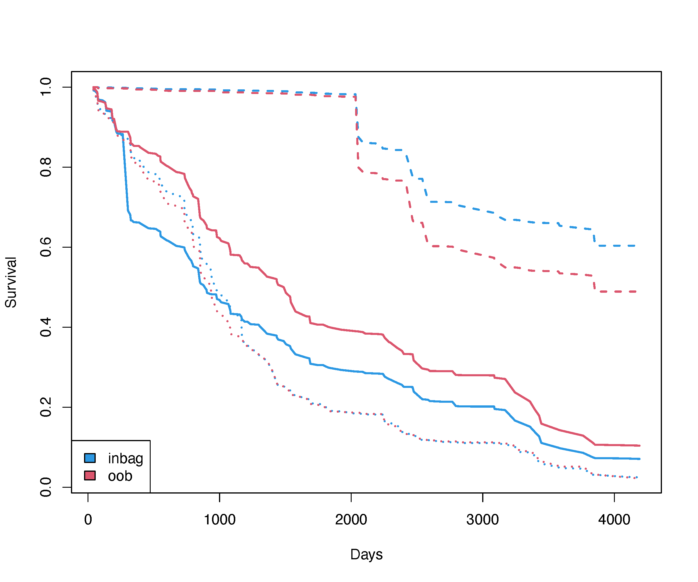

Key quantities

o$time.interest --->   event times (everything keys off this)

o$time.interest[1:5]
> [1]  41  51  71  77 110

o$predicted     --->   inbag estimated mortality
o$predicted.oob --->   OOB estimated mortality

o$predicted[1:5]
> [1] 200.83450  17.07501  76.31131  57.77577  79.27206

o$predicted.oob[1:5]
> [1] 190.04590  28.05044  66.25447  55.03181  72.55308

o$survival      --->   inbag survival estimator for each case
o$survival.oob  --->   OOB survival estimator for each case

dim(o$yvar) ## sample size (complete cases) n = 276
> [1] 276   2
length(o$time.interest)
> [1] 127
dim(o$survival)      # --->   inbag survival estimator for each case
> [1] 276 127
dim(o$survival.oob)  # --->   OOB survival estimator for each case
> [1] 276 127

Prediction error

Family	Prediction Error
Regression Quantile Regression	mean-squared error mean-squared error
Classification Imbalanced Two-Class	misclassification, Brier score G-mean, misclassification, Brier score
Survival	Harrell’s C-index (1 minus concordance)
Competing Risk	Harrell’s C-index (1 minus concordance)
Multivariate Regression Multivariate Classification Multivariate Mixed Regression Multivariate Quantile Regression	per response: same as above for Regression per response: same as above for Classification per response: same as above for Regression, Classification same as Multivariate Regression
Unsupervised sidClustering Breiman (Shi-Horvath)	none same as Multivariate Mixed Regression same as Classification

Prediction error for classification

Error rate for the chosen performance metric is always available in obj$err.rate, however any error rate can be calculated using obj$yvar with obj$predicted.oob or obj$class.oob

Misclassification error: get.misclass.error
Brier error: get.brier.error
Log-loss (cross-entropy loss): get.logloss
AUC: get.auc

Classification example: Glioma

Different prediction measures

                   (OOB) Brier score: 0.02333115
        (OOB) Normalized Brier score: 0.19053769
                           (OOB) AUC: 0.99304797
                      (OOB) Log-loss: 0.34115074
   (OOB) Requested performance error: 0.07061503, 0.06756757, 0.01149425, 0.00803213, 0.52, 0.53658537, 0.04651163, 0.11538462

tail(o$err.rate, 1)

>               all   Classic-like      Codel G-CIMP-high G-CIMP-low  LGm6-GBM   Mesenchymal-like   PA-like
> [500,] 0.07403189   0.07061503, 0.06756757, 0.01149425, 0.00803213, 0.52, 0.53658537, 0.04651163, 0.11538462

Prediction error for survival

1. Harrell’s C-error rate

Extract using obj$err.rate or get.cindex
Easy to understand
Computationally expensive
Biased in the presence of heavy censoring

2. Time-varying Brier score

Not intuitive
Computationally inexpensive: get.brier.survival
Unbiased and robust

3. Time-varying AUC (AUC-t)

Easy to understand
In principle robust
Requires sophisticated methods for calculating (see riskRegression package)

Prediction error for survival

Time-varying brier score and AUC-t for the PBC dataset

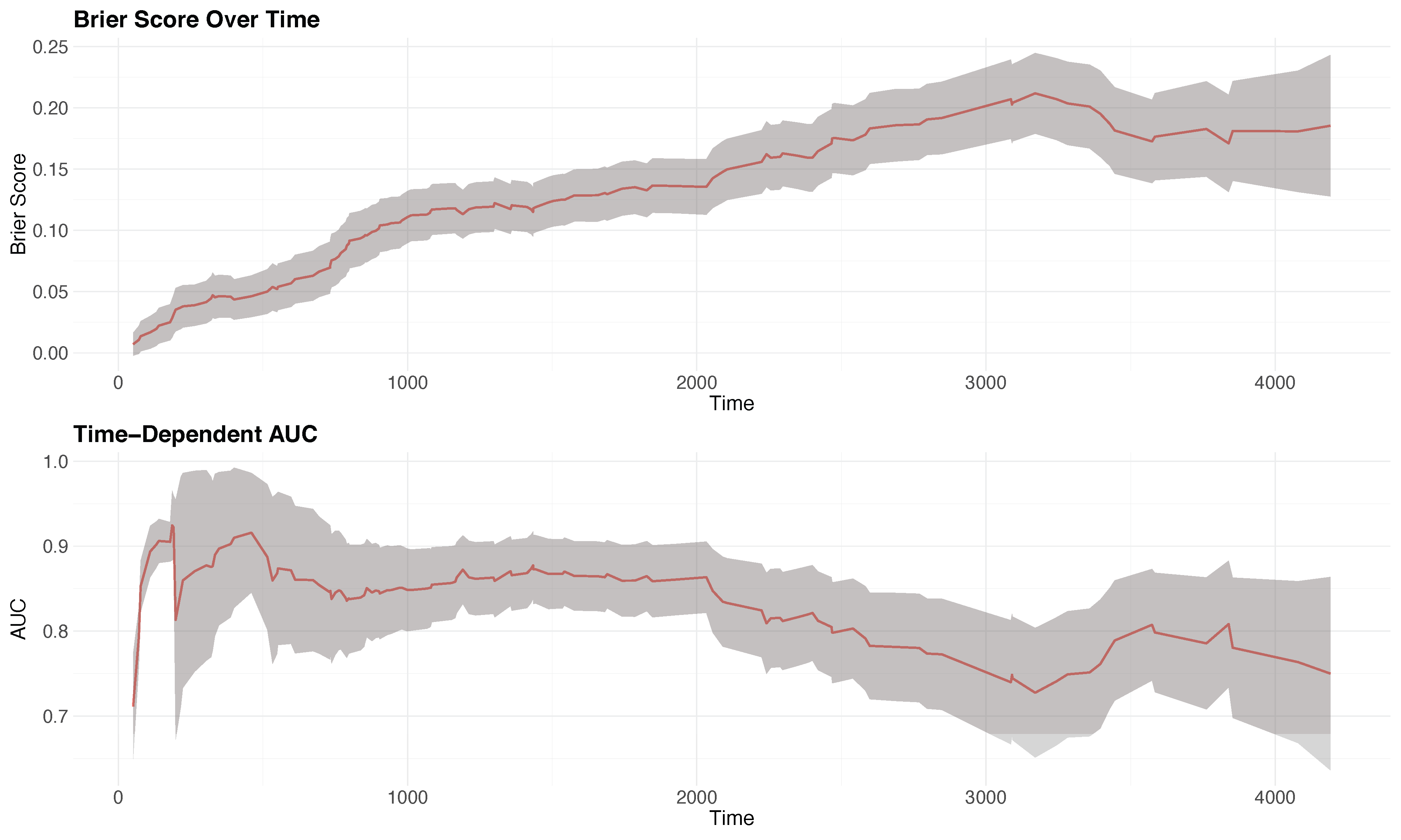
Tip:

Code generated using plot.brier.auc

Prediction

4 major ways prediction can be used

Prediction on test data: predict(object, testdata)
Prediction on “artificial data” for partial plots: plot.variable, partial
Prediction where a new data is substituted into the trained forest: predict(object, testdata, outcome = "test")
Restoring the forest: predict(object, ...)

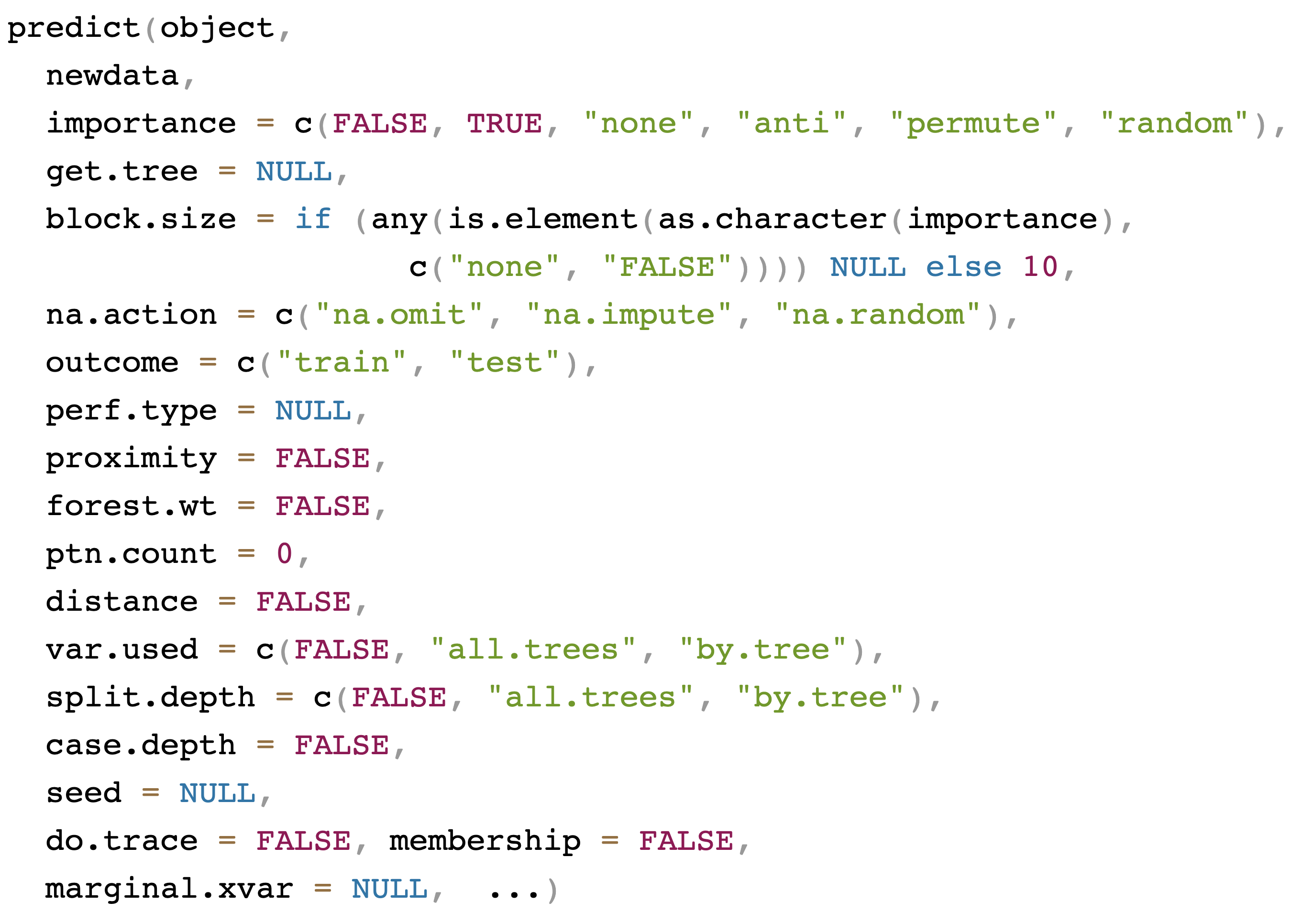
General call to predict

Prediction: canonical example

Veteran’s Administration Lung Cancer Trial

Randomized trial of two treatment regimens for lung cancer [2]

trt	celltype	time	status	karno	diagtime	age	prior
1	1	72	1	60	7	69	0
1	1	411	1	70	5	64	10
1	1	228	1	60	3	38	0
1	1	126	1	60	9	63	10
1	1	118	1	70	11	65	10
1	1	10	1	20	5	49	0
1	1	82	1	40	10	69	10
1	1	110	1	80	29	68	0
1	1	314	1	50	18	43	0
1	1	100	0	70	6	70	0

data(veteran, package = "randomForestSRC")
dim(veteran)
> [1]  137   8

Prediction: canonical example

## veteran data (with factors)
data(veteran, package = "randomForestSRC")
veteran2 <- data.frame(lapply(veteran, factor))
veteran2$time <- veteran$time
veteran2$status <- veteran$status

## split the data into unbalanced train/test data (25/75)
## the train/test data have the same levels, but different labels
train <- sample(1:nrow(veteran2), round(nrow(veteran2) * .25))

> summary(veteran2[train,])
 trt    celltype      time            status           karno      diagtime       age     prior  
 1:18   1: 8     Min.   :  3.00   Min.   :0.0000   60     :7   3      : 7   60     : 3   0 :27  
 2:16   2:10     1st Qu.: 29.25   1st Qu.:1.0000   40     :6   2      : 6   66     : 3   10: 7  
        3: 9     Median : 53.50   Median :1.0000   80     :6   5      : 3   67     : 3          
        4: 7     Mean   :104.29   Mean   :0.9412   70     :4   8      : 3   69     : 3          
                 3rd Qu.:140.25   3rd Qu.:1.0000   90     :4   1      : 2   38     : 2          
                 Max.   :389.00   Max.   :1.0000   30     :3   4      : 2   48     : 2          
                                                   (Other):4   (Other):11   (Other):18

> summary(veteran2[-train,])
 trt    celltype      time           status          karno       diagtime       age     prior  
 1:51   1:27     Min.   :  1.0   Min.   :0.000   60     :20   4      :17   63     :10   0 :70  
 2:52   2:38     1st Qu.: 21.5   1st Qu.:1.000   70     :19   2      :13   62     : 8   10:33  
        3:18     Median : 83.0   Median :1.000   80     :18   3      :11   64     : 7          
        4:20     Mean   :127.3   Mean   :0.932   30     :11   5      :11   65     : 7          
                 3rd Qu.:147.5   3rd Qu.:1.000   50     :11   11     : 5   68     : 5          
                 Max.   :999.0   Max.   :1.000   40     :10   12     : 5   70     : 5          
                                                 (Other):14   (Other):41   (Other):61

Prediction: canonical example

## train the forest and use this to predict on test data
o <- rfsrc(Surv(time, status) ~ ., veteran2[train, ]) 
pred <- predict(o, veteran2[-train , ])

> print(o)
                         Sample size: 34
                    Number of deaths: 32
                     Number of trees: 500
           Forest terminal node size: 15
       Average no. of terminal nodes: 1
No. of variables tried at each split: 3
              Total no. of variables: 6
       Resampling used to grow trees: swor
    Resample size used to grow trees: 21
                            Analysis: RSF
                              Family: surv
                      Splitting rule: logrank *random*
       Number of random split points: 10
                          (OOB) CRPS: 57.73879973
                   (OOB) stand. CRPS: 0.14842879
   (OOB) Requested performance error: 0.88246269

> print(pred)
  Sample size of test (predict) data: 103
                Number of grow trees: 500
  Average no. of grow terminal nodes: 1
         Total no. of grow variables: 6
       Resampling used to grow trees: swor
    Resample size used to grow trees: 21
                            Analysis: RSF
                              Family: surv
                                CRPS: 54.3104615
                         stand. CRPS: 0.13961558
         Requested performance error: 0.49749046

Prediction: canonical example

## even harder ... factor level not previously encountered in training
veteran3 <- veteran2[1:3, ]
veteran3$celltype <- factor(c("newlevel", "1", "3"))
pred2 <- predict(o, veteran3)
print(pred2)
>   Sample size of test (predict) data: 3
>                 Number of grow trees: 500
>   Average no. of grow terminal nodes: 1
>          Total no. of grow variables: 6
>        Resampling used to grow trees: swor
>     Resample size used to grow trees: 21
>                             Analysis: RSF
>                               Family: surv
>                                 CRPS: 60.6330452
>                          stand. CRPS: 0.15586901
>          Requested performance error: 0.5

## the unusual level is treated like a missing value but is not removed
print(pred2$xvar)
>   trt celltype karno diagtime age prior
> 1   1     <NA>    60        7  69     0
> 2   1        1    70        5  64    10
> 3   1        3    60        3  38     0

Restore

predict(object, ...)

Useful feature of predict making it possible to restore the original training forest

After tuning the forest, you can use predict to obtain: \[ \begin{array}{ll} \texttt{importance} & \text{Variable Importance (VIMP)} \\ \texttt{forest.wt} & \text{Construct your own estimator} \\ \texttt{proximity} & \text{RF proximity} \\ \texttt{distance} & \text{RF distance} \\ \texttt{get.tree} & \text{Plot a tree on your browser} \\ \texttt{var.used, split.depth} & \text{Statistics summarizing variable and tree splitting} \\ \end{array} \]

Restore

Tip

predict() can restore an object from rfsrc() with a new specification

y	cg23970089	cg25176823	cg24576735	Chr19.20co.gain	TERT.promoter.status	SNP6	U133a	grade	age	gender
Mesenchymal-like	0.36518600	0.3244530	0.03255164	No chr 19/20 gain	Mutant	Yes	Yes	G4	44	female
Mesenchymal-like	0.60246131	0.3626941	0.02215452	No chr 19/20 gain	Mutant	Yes	Yes	G4	50	male
Mesenchymal-like	0.44011951	0.3679728	0.03369096	No chr 19/20 gain	Mutant	Yes	No	G4	56	female
Classic-like	0.06834791	0.3974054	0.03623296	No chr 19/20 gain	Mutant	Yes	Yes	G4	40	female
Classic-like	0.19843219	0.2736760	0.04060163	No chr 19/20 gain	Mutant	Yes	Yes	G4	61	female

o <- rfsrc(y~., data = glioma) 
o
                         Sample size: 878
           Frequency of class labels: Classic-like=148, Codel=174, G-CIMP-high=249, G-CIMP-low=25, LGm6-GBM=41, Mesenchymal-like=215, PA-like=26
                     Number of trees: 500
           Forest terminal node size: 1
       Average no. of terminal nodes: 73.79
No. of variables tried at each split: 36
              Total no. of variables: 1241
       Resampling used to grow trees: swor
    Resample size used to grow trees: 555
                            Analysis: RF-C
                              Family: class
                      Splitting rule: gini *random*
       Number of random split points: 10
                   (OOB) Brier score: 0.02270041
        (OOB) Normalized Brier score: 0.18538666
                           (OOB) AUC: 0.99380046
                      (OOB) Log-loss: 0.33499374
   (OOB) Requested performance error: 0.06719818, 0.04054054, 0.01149425, 0.00803213, 0.52, 0.48780488, 0.05581395, 0.15384615

Confusion matrix:

                  predicted
  observed         Classic-like Codel G-CIMP-high G-CIMP-low LGm6-GBM Mesenchymal-like PA-like class.error
  Classic-like              143     0           0          0        0                5       0      0.0338
  Codel                       0   172           2          0        0                0       0      0.0115
  G-CIMP-high                 0     2         247          0        0                0       0      0.0080
  G-CIMP-low                  0     0          13         12        0                0       0      0.5200
  LGm6-GBM                    0     0           1          0       21               19       0      0.4878
  Mesenchymal-like           12     0           0          0        0              203       0      0.0558
  PA-like                     0     0           0          0        0                4      22      0.1538

      (OOB) Misclassification rate: 0.06605923

Random-classifier baselines (uniform):
   Brier: 0.12244898   Normalized Brier: 1   Log-loss: 1.94591015

p <- predict(o, perf.type = "brier") 
p
  Sample size of test (predict) data: 878
                Number of grow trees: 500
  Average no. of grow terminal nodes: 73.79
         Total no. of grow variables: 1241
       Resampling used to grow trees: swor
                            Analysis: RF-C
                              Family: class
                         Brier score: 0.02270041
              Normalized Brier score: 0.18538666
                                 AUC: 0.99380046
                            Log-loss: 0.33499374
         Requested performance error: 0.18538666, 0.03943965, 0.01378517, 0.02434763, 0.01397218, 0.02309749, 0.06058674, 0.0101578
         
Confusion matrix:

                  predicted
  observed         Classic-like Codel G-CIMP-high G-CIMP-low LGm6-GBM Mesenchymal-like PA-like class.error
  Classic-like              143     0           0          0        0                5       0      0.0338
  Codel                       0   172           2          0        0                0       0      0.0115
  G-CIMP-high                 0     2         247          0        0                0       0      0.0080
  G-CIMP-low                  0     0          13         12        0                0       0      0.5200
  LGm6-GBM                    0     0           1          0       21               19       0      0.4878
  Mesenchymal-like           12     0           0          0        0              203       0      0.0558
  PA-like                     0     0           0          0        0                4      22      0.1538

      (OOB) Misclassification rate: 0.06605923

Random-classifier baselines (uniform):
   Brier: 0.12244898   Normalized Brier: 1   Log-loss: 1.94591015

Restore

Create your own estimator for regression

## create your own estimator for regression
o <- rfsrc(mpg~.,mtcars)
fwt <- predict(o, forest.wt="oob")$forest.wt
yhat <- c(fwt %*% o$yvar)

## compare to the OOB ensemble
print(summary(yhat - o$predicted.oob))
      Min.    1st Qu.     Median       Mean    3rd Qu.       Max. 
-3.908e-14 -1.643e-14 -1.066e-14 -1.060e-14 -3.553e-15  1.066e-14
      
## compare prediction error to OOB ensemble
print(o)

                        Sample size: 32
                     Number of trees: 500
           Forest terminal node size: 5
       Average no. of terminal nodes: 3.476
No. of variables tried at each split: 4
              Total no. of variables: 10
       Resampling used to grow trees: swor
    Resample size used to grow trees: 20
                            Analysis: RF-R
                              Family: regr
                      Splitting rule: mse *random*
       Number of random split points: 10
                     (OOB) R squared: 0.76585425
   (OOB) Requested performance error: 8.50513415

print(mean((yhat - o$yvar)^2))
8.505134

Partial plots

Partial plots are used to understand the effect of a feature on the outcome and are essentially prediction tools

Consider nonparametric regression \[ F(x_1,\ldots,x_p) = E[Y|(x_1,\ldots,x_p)] \] To study variable $j$ we plot $F_j(x)$ over $x$ where \[ F_j(x) = \frac{1}{n}\sum_{i=1}^nF_{\!\text{ens}}(x_1=x_{i1},\ldots,\color{red}{x_j=x},\color{black}\ldots,x_p=x_{ip}) \] and \[ \Bigg\{\Big(x_1=x_{i1},\ldots,\color{red}{x_j=x}\color{black},\ldots,x_p=x_{ip}\Big):\hskip10pt i=1,\ldots,n\Bigg\} \] are “test” data values equal to the training data but where coordinate $j$ is set to $x$

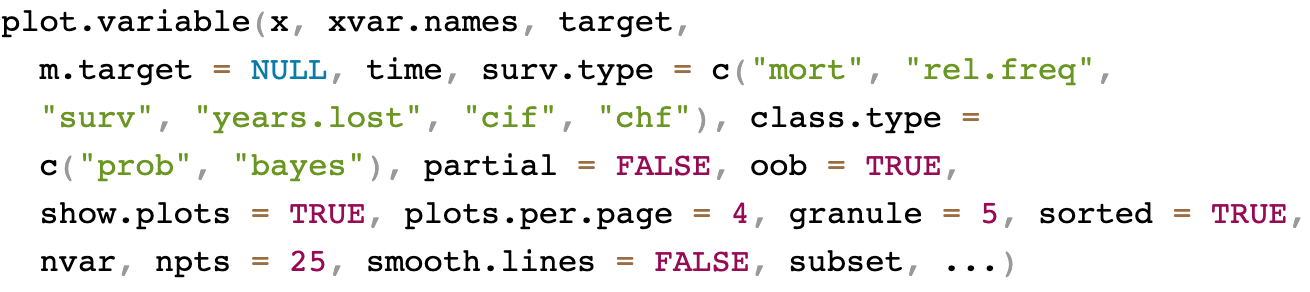
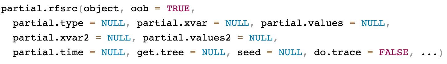
General call to plot.variable

General call to partial

Survival example: peakVO2

The data involve 2231 patients with systolic heart failure who underwent cardiopulmonary stress testing at the Cleveland Clinic. The primary end point was all-cause death. In total, 39 variables were measured for each patient, including baseline clinical values and exercise stress test results. A key variable of interest is peak VO2 (mL/kg per min), the peak respiratory exchange ratio [3]

ttodead	died	bun	sodium	hgb	glucose	male	crcl	age	betablok	acei	angioten.II	anti.arrhy	anti.coag	aspirin	digoxin
1.207392	0	25.00000	141.0000	14.60000	89.00000	1	49.92778	74	1	0	1	1	1	1	0
3.611225	0	20.00000	138.0000	13.10000	90.00000	0	60.35000	77	1	1	0	0	0	1	1
0.238193	1	29.68983	139.8368	12.87517	98.74435	1	33.61172	79	0	0	0	0	0	1	1
10.513347	0	27.87734	139.4590	13.16225	136.87414	1	69.25114	67	0	1	0	0	1	0	1
3.712526	1	39.00000	143.0000	12.50000	104.00000	1	44.67685	79	1	0	1	0	0	1	0

data(peakVO2, package = "randomForestSRC") 
dim(peakVO2)
> [1]  2231   41

Survival example: peakVO2

We can use plot.variable to visualize $F_j(x)$

o <- rfsrc(Surv(ttodead,died)~., peakVO2)
## partial effect for age
plot.variable(o, surv.type = "surv", xvar.names = "age", 
              time = 2, partial = TRUE)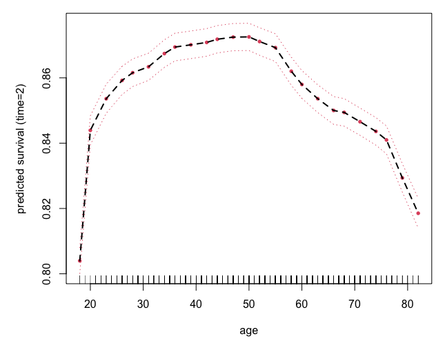

Survival example: peakVO2


## partial effect for age
plot.variable(o, surv.type = "surv", xvar.names = "age", 
              smooth.lines = TRUE,
              time = 2, partial = TRUE)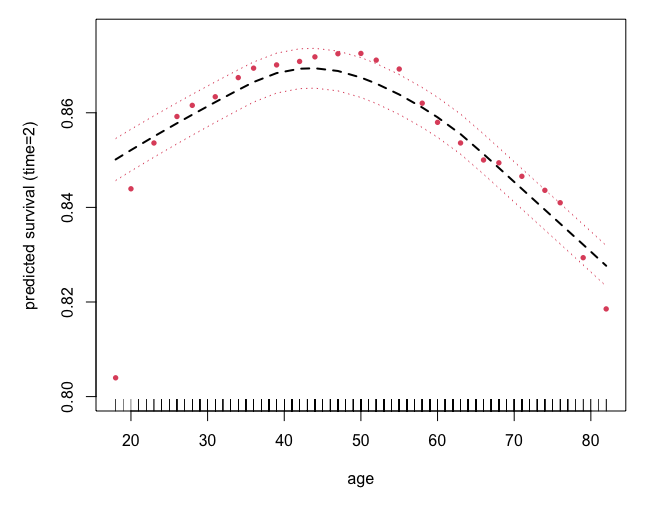

Survival example: peakVO2


## partial effect for age
plot.variable(o, surv.type = "rel.freq", xvar.names = "age", 
              smooth.lines = TRUE,
              partial = TRUE)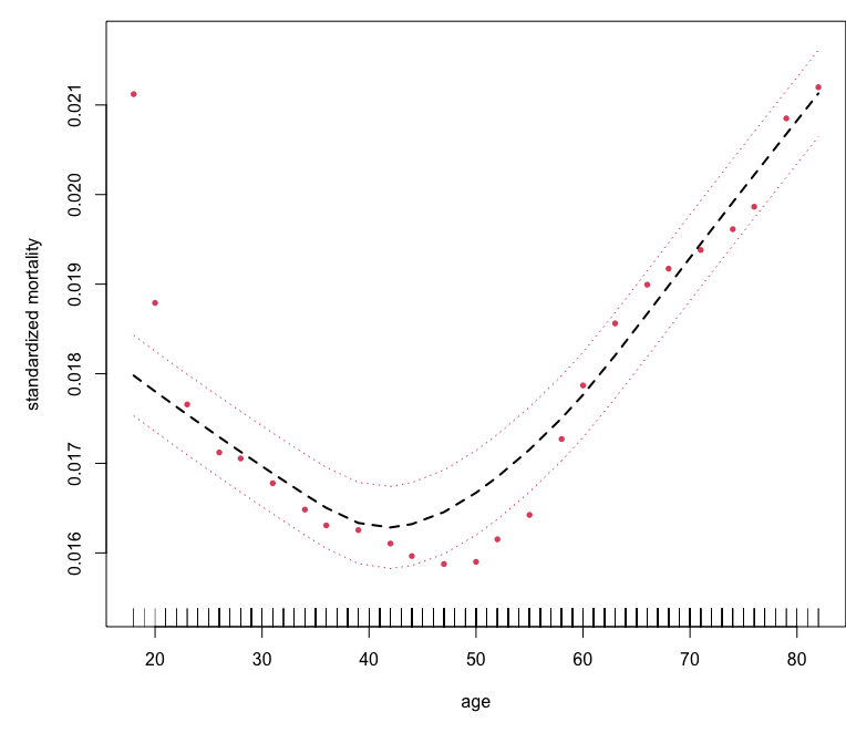

Survival example: peakVO2

We can use partial and get.partial.plot.data to obtain values of $F_j(x)$

## partial effect of peak V02 on mortality

partial.o <- partial(o,
                     partial.type = "mort",
                     partial.xvar = "peak.vo2",
                     partial.values = o$xvar$peak.vo2,
                     partial.time = o$time.interest)
pdta.m <- get.partial.plot.data(partial.o)

## partial effect of peak V02 on survival
pvo2 <- quantile(o$xvar$peak.vo2)
partial.o <- partial(o,
                     partial.type = "surv",
                     partial.xvar = "peak.vo2",
                     partial.values = pvo2,
                     partial.time = o$time.interest)
pdta.s <- get.partial.plot.data(partial.o)

## compare the two plots
par(mfrow=c(1,2))    

plot(lowess(pdta.m$x, pdta.m$yhat, f = 2/3),
     type = "l", xlab = "peak VO2", ylab = "adjusted mortality")
rug(o$xvar$peak.vo2)

matplot(pdta.s$partial.time, t(pdta.s$yhat), type = "l", lty = 1,
        xlab = "years", ylab = "peak VO2 adjusted survival")
legend("bottomleft", legend = paste0("peak VO2 = ", pvo2),
       bty = "n", cex = .75, fill = 1:5)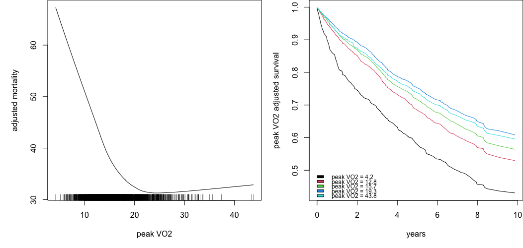

Outline

Part I: Training

Quick start
Data structures allowed
Training (grow) with examples
(regression, classification, survival)

Part II: Inference and Prediction

Inference (OOB)
Prediction Error
Prediction
Restore
Partial Plots

Part III: Variable Selection

VIMP
Subsampling (Confidence Intervals)
Minimal Depth
VarPro

Part IV: Advanced Examples

Class Imbalanced Data
Competing Risks
Multivariate Forests
Missing data imputation

References

1. Efron B, Tibshirani R. Improvements on cross-validation: The 632+ bootstrap method. Journal of the American Statistical Association. 1997;92:548–60.

2. Kalbfleisch JD, Prentice RL. The statistical analysis of failure time data. John Wiley & Sons; 1980.

3. Hsich E, Gorodeski EZ, Blackstone EH, Ishwaran H, Lauer MS. Identifying important risk factors for survival in patient with systolic heart failure using random survival forests. Circulation: Cardiovascular Quality and Outcomes. 2011;4:39–45.

trt	celltype	time	status	karno	diagtime	age	prior
1	1	72	1	60	7	69	0
1	1	411	1	70	5	64	10
1	1	228	1	60	3	38	0
1	1	126	1	60	9	63	10
1	1	118	1	70	11	65	10
1	1	10	1	20	5	49	0
1	1	82	1	40	10	69	10
1	1	110	1	80	29	68	0
1	1	314	1	50	18	43	0
1	1	100	0	70	6	70	0

trt	celltype	time	status	karno	diagtime	age	prior
1	1	72	1	60	7	69	0
1	1	411	1	70	5	64	10
1	1	228	1	60	3	38	0
1	1	126	1	60	9	63	10
1	1	118	1	70	11	65	10
1	1	10	1	20	5	49	0
1	1	82	1	40	10	69	10
1	1	110	1	80	29	68	0
1	1	314	1	50	18	43	0
1	1	100	0	70	6	70	0

trt	celltype	time	status	karno	diagtime	age	prior
1	1	72	1	60	7	69	0
1	1	411	1	70	5	64	10
1	1	228	1	60	3	38	0
1	1	126	1	60	9	63	10
1	1	118	1	70	11	65	10
1	1	10	1	20	5	49	0
1	1	82	1	40	10	69	10
1	1	110	1	80	29	68	0
1	1	314	1	50	18	43	0
1	1	100	0	70	6	70	0