| age | betablok | dilver | nifed | acei | angioten.II | anti.arrhy | anti.coag | aspirin | digoxin | nitrates | vasodilator | diuretic.loop | diuretic.thiazide | diuretic.potassium.spar | lipidrx.statin | insulin | surgery.pacemaker | surgery.cabg | surgery.pci | surgery.aicd.implant | resting.systolic.bp | resting.hr | smknow | q.wave.mi | bmi | niddm | lvef.metabl | peak.rer | peak.vo2 | interval | cad | died | ttodead | bun | sodium | hgb | glucose | male | black | crcl |
|---|---|---|---|---|---|---|---|---|---|---|---|---|---|---|---|---|---|---|---|---|---|---|---|---|---|---|---|---|---|---|---|---|---|---|---|---|---|---|---|---|
| 61 | 1 | 0 | 1 | 1 | 0 | 0 | 0 | 1 | 0 | 1 | 0 | 0 | 1 | 0 | 1 | 0 | 0 | 1 | 1 | 0 | 100 | 75 | 0 | 1 | 28.68956 | 0 | 30 | 0.97 | 4.2 | 360 | 1 | 0 | 2.354552 | 20 | 141 | 14.3 | 90 | 1 | 0 | 71.24107 |
Tree-Based Machine Learning Methods for Prediction and Variable Selection
Part III
Hemant Ishwaran and Min Lu
University of Miami
University of Miami
Variable selection
We will discuss 4 different methods
- Permutation Variable Importance (VIMP)
- Subsampling for Confidence Intervals
- Minimal Depth
- VarPro
Permutation importance
Idea
In the OOB cases for a tree, randomly permute all values of the \(j\)th variable. Put these new covariate values down the tree and compute a new internal error rate. The amount by which this new error exceeds the original OOB error is defined as the importance of the \(j\)th variable for the tree. Averaging over the forest yields VIMP.
— Measure 1 (Manual On Setting Up, Using, And Understanding Random Forests V3.1
Learn more [1]: http://randomforestsrc.org/articles/vimp.html
OOB explanation
The tree OOB error rate is \[ \frac{1}{\# O_{ib}}\sum_{i\in O_{ib}} L(Y_i,h^*_b(\mathbf{x}_i)) \]
Permute (perturb) the \(j\) covariate feature for \(i\) to obtain \(\mathbf{x}^{*(j)}_i\)
The tree VIMP is therefore \[ \frac{1}{\# O_{ib}}\sum_{i\in O_{ib}} L(Y_i,h^*_b(\mathbf{x}^{*(j)}_i)) - \frac{1}{\# O_{ib}}\sum_{i\in O_{ib}} L(Y_i,h^*_b(\mathbf{x}_i)) \]
Averaging over trees gives VIMP. Large values identify important variables (negative values can occur!)
OOB explanation
Different VIMP in the package
Obtaining VIMP using the package
During training:
rfsrc(mpg~., importance="permute")$importance
rfsrc(mpg~., importance="permute", block.size=10)$importance
Using restore:
predict(obj, importance="permute")$importance
predict(obj, importance="permute", block.size=10)$importance
Using vimp:
vimp also permits joint VIMP
General call to vimp
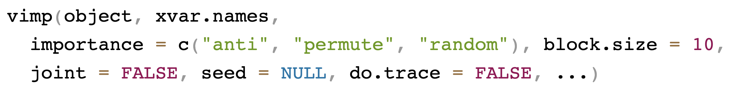
## VIMP for all variables
iris.obj <- rfsrc(Species ~ ., data = iris)
> print(vimp(iris.obj, importance = "permute")$importance)
                    all setosa versicolor virginica
Sepal.Length 0.01547102 0.0196     0.0168    0.0096
Sepal.Width  0.00471908 0.0108    -0.0056    0.0088
Petal.Length 0.20141104 0.2568     0.2212    0.1208
Petal.Width 0.23262283 0.3220 0.2640 0.1048VIMP illustration using peakVO2
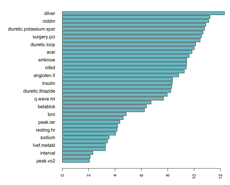
We have \(n=2231\) cardiovascular patients with systolic heart failure and all underwent cardiopulmonary stress testing. The outcome is all cause mortality (mean follow-up of 5 years, 742 patients died). Baseline characteristics and exercise stress test results were recorded (\(p=39\)).
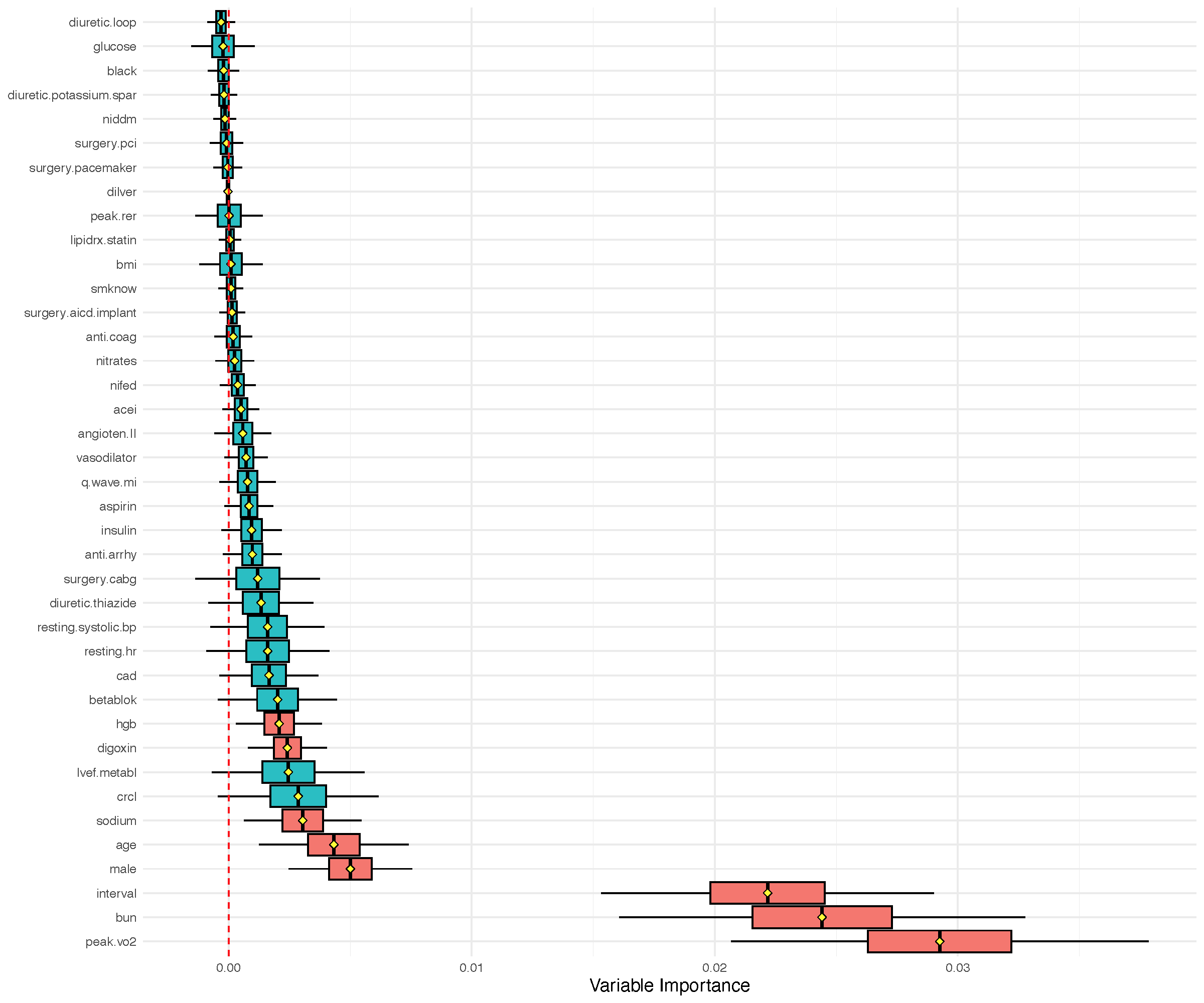
VIMP illustration using peakVO2
Confidence intervals for VIMP
VIMP standard error and CI are obtained using subsampling
Subsampling samples data without replacement where the subsample size \(m\) is substantially smaller than \(n\); eg: \[ m=\sqrt{n}=\sqrt{2231}\approx 48\ll n=2231 \]
CI are obtained using normal approximations \[ \texttt{vimp} \pm z_{\alpha/2} \hat{\sigma} \] where \(\hat{\sigma}\) is the subsampled standard error estimator[2, 3]
VIMP for regression: Iowa housing
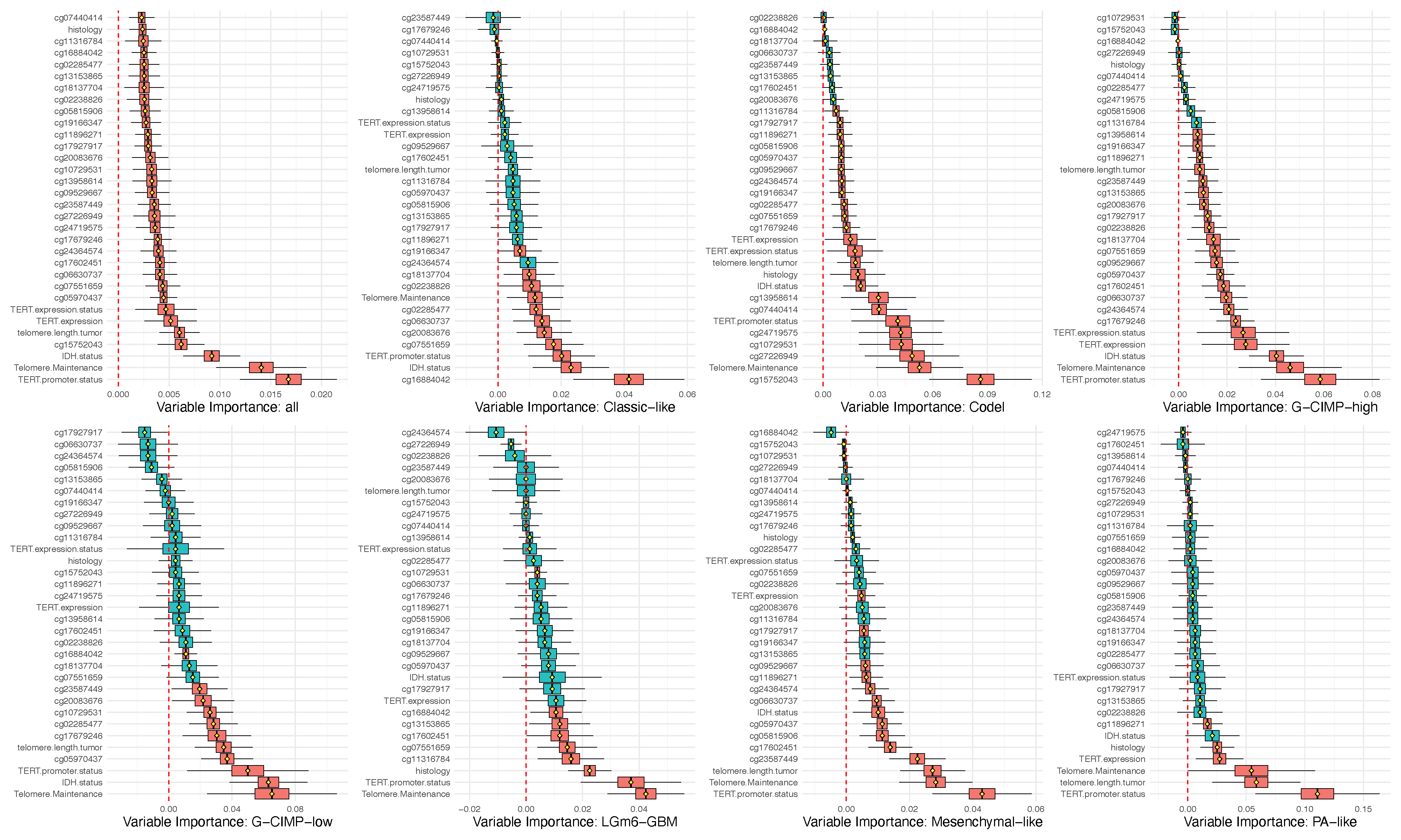
VIMP for classification example: Glioma
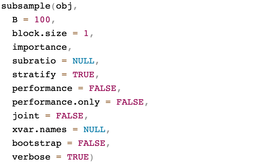
General call to subsample
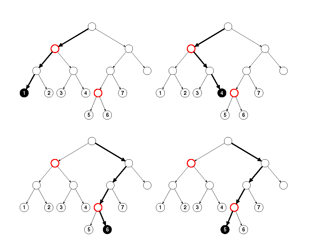
Minimal depth
Measures importance of a variable by how close it splits to the root
Pros:
- Much faster
- Works in all settings for any type of tree
- Doesn’t depend on prediction error
Cons:
- Threshold value can be sensitive and relies on assumptions
Learn more [4]: https://www.randomforestsrc.org/articles/minidep.html
Minimal depth
General call to max.subtree

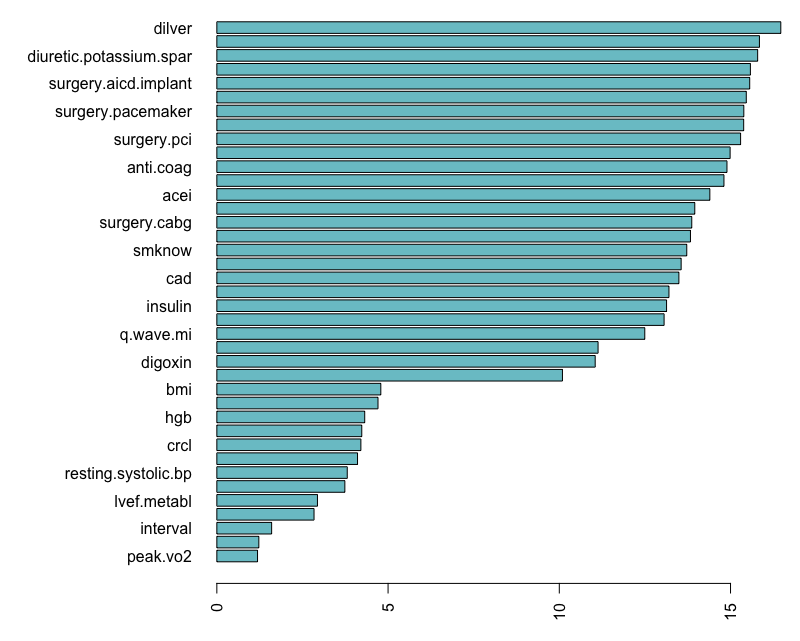
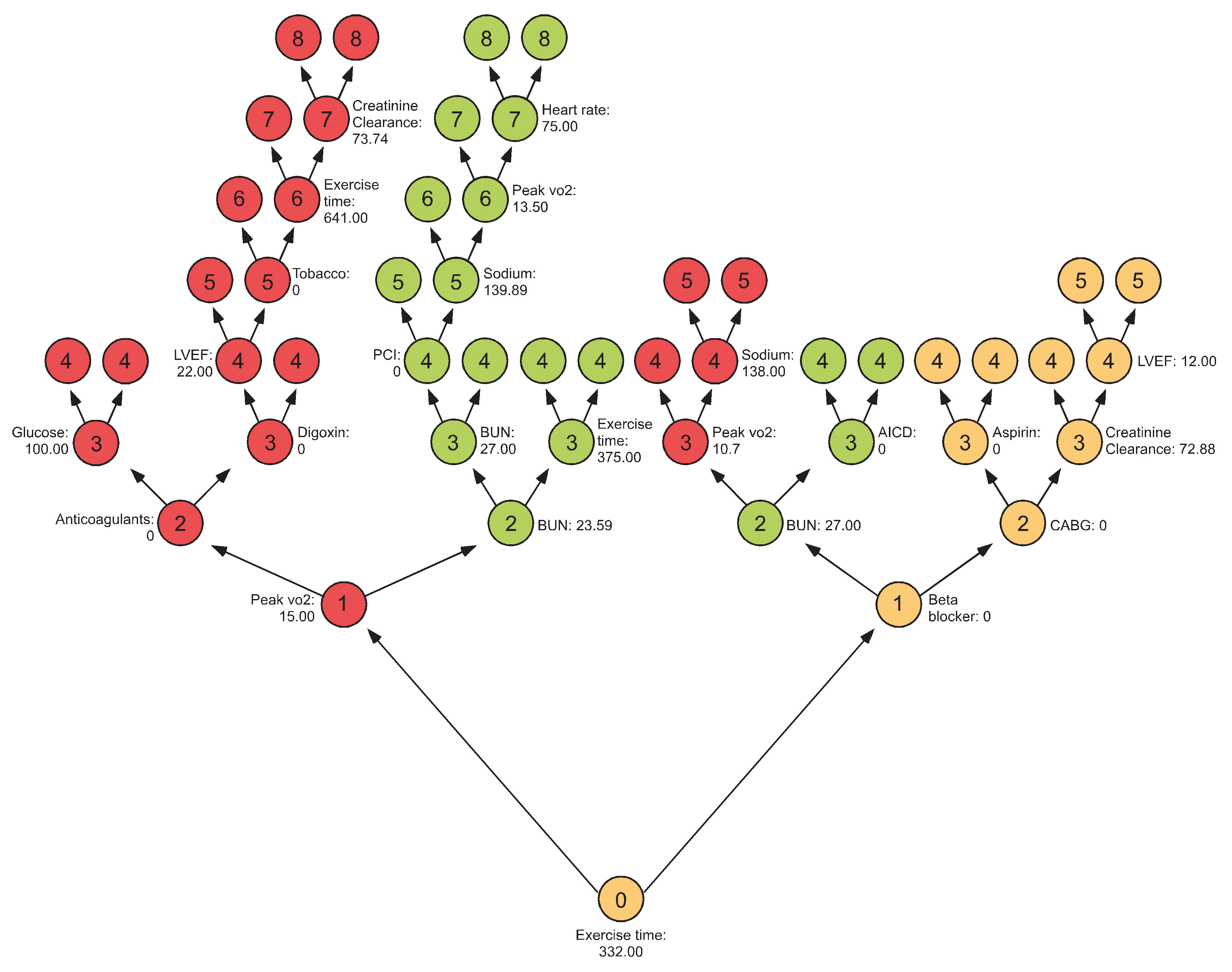
Minimal depth illustration using peakVO2
Minimal depth illustration using peakVO2
VarPro
Permutation VIMP creates “artificial” data which can impact performance in correlated settings
VarPro
Permutation VIMP creates “artificial” data which can impact performance in correlated settings
Consider a patient in the peakVO2 dataset
| bun | interval | peak.vo2 |
|---|---|---|
| 20 | 360 | 4.2 |
Suppose peak.vo2 is permuted for calculating VIMP
| age | betablok | dilver | nifed | acei | angioten.II | anti.arrhy | anti.coag | aspirin | digoxin | nitrates | vasodilator | diuretic.loop | diuretic.thiazide | diuretic.potassium.spar | lipidrx.statin | insulin | surgery.pacemaker | surgery.cabg | surgery.pci | surgery.aicd.implant | resting.systolic.bp | resting.hr | smknow | q.wave.mi | bmi | niddm | lvef.metabl | peak.rer | peak.vo2 | interval | cad | died | ttodead | bun | sodium | hgb | glucose | male | black | crcl |
|---|---|---|---|---|---|---|---|---|---|---|---|---|---|---|---|---|---|---|---|---|---|---|---|---|---|---|---|---|---|---|---|---|---|---|---|---|---|---|---|---|
| 61 | 1 | 0 | 1 | 1 | 0 | 0 | 0 | 1 | 0 | 1 | 0 | 0 | 1 | 0 | 1 | 0 | 0 | 1 | 1 | 0 | 100 | 75 | 0 | 1 | 28.68956 | 0 | 30 | 0.97 | 43.8 | 360 | 1 | 0 | 2.354552 | 20 | 141 | 14.3 | 90 | 1 | 0 | 71.24107 |
| bun | interval | peak.vo2 |
|---|---|---|
| 20 | 360 | 43.8 |
> summary(peakVO2[,c("bun","interval", "peak.vo2")])
      bun             interval         peak.vo2
 Min.   :  4.322   Min.   :  21.0   Min.   : 4.20
 1st Qu.: 17.000   1st Qu.: 345.0   1st Qu.:12.80
 Median : 23.000   Median : 480.0   Median :15.70
 Mean   : 25.278   Mean   : 503.3   Mean   :16.27
 3rd Qu.: 29.334   3rd Qu.: 641.0   3rd Qu.:19.30
 Max.   :129.000   Max.   :1415.0   Max.   :43.80
Permuting the data can create implausible values
VarPro
Permutation VIMP creates “artificial” data which can impact performance in correlated settings
VarPro works directly with the observed data creating a test statistic [5]
For each tree branch (a rule), the rule is released along the coordinate \(j\). Importance equals the difference between the test statistic for the original rule to the released rule
VarPro: pros and cons
Pros:
- Much faster
- Much better for correlated problems
- User specified test statistics
- Doesn’t depend on prediction error
- Tree guided rules can be specified by the user
- Sparsity property
Cons:
- Importance value does not have an intuitive interpretation
General call to varpro
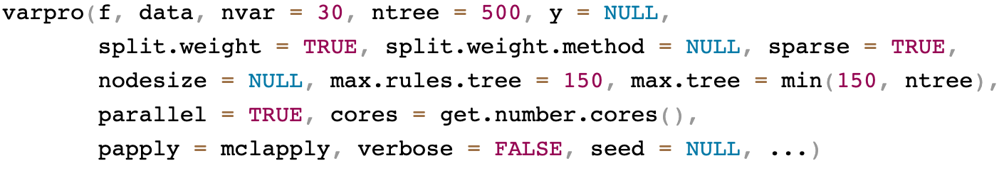
VarPro canonical illustration
## varpro canonical call
o <-varpro(Surv(ttodead, died)~., peakVO2)
importance(o)

## cv.varpro canonical call
o.cv <- cv.varpro(Surv(ttodead, died)~., peakVO2)
o.cv
> importance(o)
z
bun 2.02513310
peak.vo2 1.74518274
interval 1.68998740
male 1.47082361
betablok 1.33132611
sodium 1.03537549
lvef.metabl 0.66984194
hgb 0.66657629
age 0.61875665
surgery.cabg 0.58904406
digoxin 0.53693744
resting.systolic.bp 0.48385996
resting.hr 0.18797789
crcl 0.15568756
insulin 0.04772794
bmi 0.04587999
aspirin 0.00000000
diuretic.thiazide 0.00000000VarPro canonical illustration
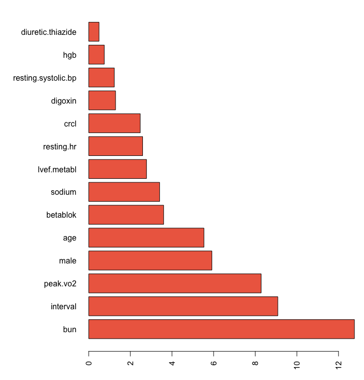
> o.cv
$imp
variable z
1 bun 12.765690
2 interval 9.084990
3 peak.vo2 8.284743
4 male 5.918617
5 age 5.537937
6 betablok 3.600902
7 sodium 3.408508
8 lvef.metabl 2.776717
9 resting.hr 2.590353
10 crcl 2.476236
11 digoxin 1.289895
$imp.conserve
variable z
1 bun 12.765690
2 interval 9.084990
3 peak.vo2 8.284743
4 male 5.918617
5 age 5.537937
6 betablok 3.600902
7 sodium 3.408508
8 lvef.metabl 2.776717
9 resting.hr 2.590353
10 crcl 2.476236
$imp.liberal
variable z
1 bun 12.7656902
2 interval 9.0849901
3 peak.vo2 8.2847426
4 male 5.9186167
5 age 5.5379366
6 betablok 3.6009023
7 sodium 3.4085085
8 lvef.metabl 2.7767175
9 resting.hr 2.5903526
10 crcl 2.4762361
11 digoxin 1.2898949
12 resting.systolic.bp 1.2290245
13 hgb 0.7475712
14 diuretic.thiazide 0.4964589
$err
zcut nvar err sd
[1,] 0.1000000 14 0.3120663 0.007186951
[2,] 0.5265306 13 0.3137940 0.004717065
[3,] 0.7591837 12 0.3141295 0.004068593
[4,] 1.2632653 11 0.3099739 0.003270832
[5,] 1.3020408 10 0.3123732 0.004680203
$zcut
[1] 1.263265
$zcut.conserve
[1] 1.302041
$zcut.liberal
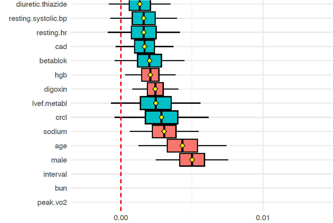
[1] 0.1VarPro canonical illustration
VarPro canonical illustration
VarPro high-dimensional example
van de Vijver Microarray Breast Cancer
Gene expression profiling for predicting clinical outcome of breast cancer [6]. Microarray breast cancer data set of 4707 expression values on 78 patients with survival information
| Time | Censoring | AA555029_RC | AA598803_RC | AB002301 | AB002308 | AB002331 | AB002351 | AB002445 | AB002448 | AB004064 | AB004857 | AB006625 | AB006628 | AB006746 | AB007458 | AB007855 | AB007857 | AB007883 | AB007888 |
|---|---|---|---|---|---|---|---|---|---|---|---|---|---|---|---|---|---|---|---|
| 12.53 | 0 | -0.5049331 | -0.2425008 | -0.199315682 | 0.90024251 | 0.6311663 | -0.6012690 | 0.44181645 | -0.26575425 | -2.80370736 | 0.13287713 | -1.1427432 | -0.52818656 | -0.97000301 | 0.32222703 | 0.41856295 | 1.1294556 | 0.4218849 | -0.16941833 |
| 6.44 | 0 | -0.5879813 | 0.4384945 | -0.621200562 | 0.09301399 | 0.9500715 | -1.4849019 | 0.21924725 | 0.14616483 | 0.08637013 | 0.59130323 | 1.1859283 | -0.70424873 | -0.62120056 | 0.33883667 | 0.05979471 | 0.1129456 | 0.4484603 | -0.05979471 |
| 10.66 | 0 | -0.3521244 | -0.2258911 | 0.006643856 | 0.13952097 | -0.7275022 | -1.0430855 | -0.27572003 | -0.49496728 | 0.56140584 | 0.71089262 | 1.2424011 | -0.77068734 | 1.12613368 | -0.38534367 | -0.23253496 | -0.6079128 | -0.6909611 | -1.13609946 |
| 13.00 | 0 | -0.4750357 | 0.5016111 | -0.671029449 | 0.76404345 | -0.9234960 | -1.9267184 | -0.01993157 | 0.09301399 | 0.41524100 | 0.24250075 | -0.9002425 | 0.07972627 | -0.43517259 | 0.05315085 | -1.56795001 | -0.9102083 | -0.2823639 | -0.12623326 |
| 11.98 | 0 | -0.1660964 | 0.1361991 | 0.989934564 | 0.62452251 | 0.9168522 | -1.4550045 | 0.07972627 | 0.77733117 | 0.19267184 | -0.37205595 | -0.9700030 | -0.41856295 | -0.07640435 | -0.20263761 | 0.54147428 | -0.1926718 | 0.4584261 | 0.71089262 |
| 11.16 | 0 | -0.8935987 | -0.1361991 | 0.438494503 | 0.56140584 | -0.4551041 | -1.5679500 | -0.42852873 | 0.28568581 | -0.25911039 | 0.47835764 | 2.2356577 | -0.59130323 | -0.83712590 | 0.48500150 | -0.03321928 | 1.2457230 | -0.1195894 | -0.27239811 |
| 10.14 | 0 | -0.4916454 | -0.5746936 | -0.289007753 | 0.16941833 | 0.9135302 | -0.1129456 | 0.20928147 | -0.47171378 | 0.52818656 | 0.03321928 | -0.8138724 | -0.68431717 | -0.52486461 | 0.07640435 | 0.69096106 | 1.3686343 | -0.1959938 | -0.19599375 |
| 8.80 | 0 | -0.4650699 | -0.2956516 | -0.385343671 | -0.26907617 | -0.3587682 | -1.4815799 | -0.97664684 | -0.87366706 | 0.60126901 | -0.42188486 | -1.6543202 | -0.57137161 | 1.12613368 | -0.57137161 | -0.98661262 | -1.3088397 | -1.0497292 | -0.52486461 |
VarPro high-dimensional example
## van de Vijver Microarray Breast Cancer
## high dimensional survival example using different split-weights
## illustrates guided trees

data(vdv, package = "randomForestSRC")
f <- as.formula(Surv(Time, Censoring)~.)

## lasso only
importance(varpro(f, vdv, split.weight.method = "lasso"))

## lasso and vimp
importance(varpro(f, vdv, split.weight.method = "lasso vimp"))

## lasso, vimp and shallow trees
importance(varpro(f, vdv, split.weight.method = "lasso vimp tree"))

## store the original vdv 70 gene signature in object nms
## compare methods using 25 runs:
rO <- lapply(1:25, function(b) {
  cat("replication:", b, "\n")
  o1 <- varpro(f, vdv, split.weight.method = "lasso")
  o2 <- varpro(f, vdv, split.weight.method = "lasso vimp")
  o3 <- varpro(f, vdv, split.weight.method = "lasso vimp tree")
  o4 <- varpro(f, vdv, split.weight.method = "lasso vimp", sparse = FALSE)
  list("lasso"=intersect(nms,get.orgvimp(o1)$variable),
       "lasso.vimp"=intersect(nms,get.orgvimp(o2)$variable),
       "lasso.vimp.tree"=intersect(nms,get.orgvimp(o3)$variable),
       "lasso.vimp.sparseoff"=intersect(nms,get.orgvimp(o4)$variable))
})
VarPro high-dimensional example
data(vdv, package = "randomForestSRC")
f <- as.formula(Surv(Time, Censoring)~.)

## lasso only
importance(varpro(f, vdv, split.weight.method = "lasso"))

## lasso and vimp
importance(varpro(f, vdv, split.weight.method = "lasso vimp"))

## lasso, vimp and shallow trees
importance(varpro(f, vdv, split.weight.method = "lasso vimp tree"))

## store the original vdv 70 gene signature in object nms
## compare methods using 25 runs:
rO <- lapply(1:25, function(b) {
  cat("replication:", b, "\n")
  o1 <- varpro(f, vdv, split.weight.method = "lasso")
  o2 <- varpro(f, vdv, split.weight.method = "lasso vimp")
  o3 <- varpro(f, vdv, split.weight.method = "lasso vimp tree")
  o4 <- varpro(f, vdv, split.weight.method = "lasso vimp", sparse = FALSE)
  list("lasso"=intersect(nms,get.orgvimp(o1)$variable),
       "lasso.vimp"=intersect(nms,get.orgvimp(o2)$variable),
       "lasso.vimp.tree"=intersect(nms,get.orgvimp(o3)$variable),
       "lasso.vimp.sparseoff"=intersect(nms,get.orgvimp(o4)$variable))
})
Intersection with VDV 70 gene signature
$lasso
[1] "AF201951" "AL080059"
[3] "Contig25991" "Contig28552_RC"
[5] "NM_000436" "NM_003748"
[7] "NM_005915" "NM_006681"
[9] "NM_020974"
$lasso.vimp
[1] "AL137718" "Contig25991"
[3] "Contig28552_RC" "Contig51464_RC"
[5] "Contig55377_RC" "NM_000436"
[7] "NM_003239" "NM_003748"
[9] "NM_005915" "NM_006681"
[11] "NM_016448" "NM_020974"
$lasso.vimp.tree
[1] "AA555029_RC" "AF201951"
[3] "AL080059" "Contig25991"
[5] "Contig28552_RC" "Contig55377_RC"
[7] "NM_000436" "NM_003748"
[9] "NM_005915" "NM_006117"
[11] "NM_006681" "NM_016448"
[13] "NM_020974"
$lasso.vimp.sparseoff
[1] "AF201951" "AF257175"
[3] "AL080059" "AL137718"
[5] "Contig25991" "Contig28552_RC"
[7] "Contig40831_RC" "Contig48328_RC"
[9] "Contig51464_RC" "Contig55377_RC"
[11] "Contig63102_RC" "NM_002916"
[13] "NM_003239" "NM_003748"
[15] "NM_005915" "NM_006117"
[17] "NM_006681" "NM_016448"
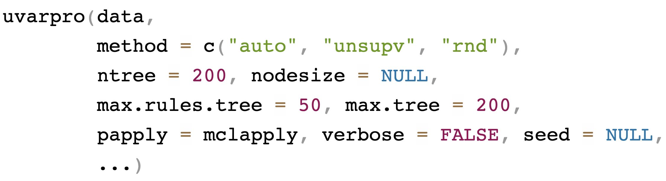
[19] "NM_020974" Unsupervised Variable Selection (UVarPro)
General call to uvarpro [7]
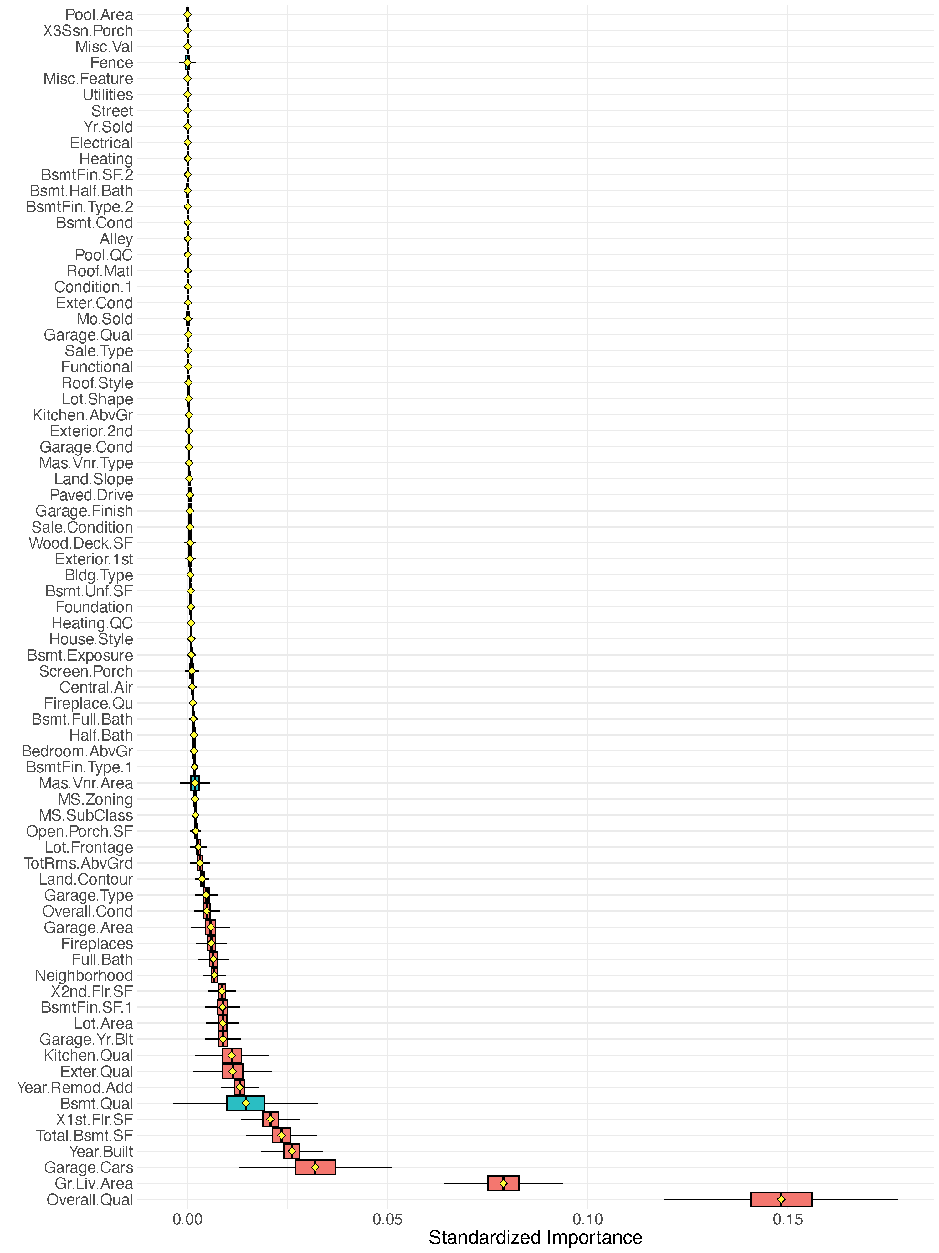
UVarPro illustration with Iowa housing
## load the data
data(housing, package = "randomForestSRC")

## rough impute

## convert factors to numerical
iowa <- randomForestSRC:::get.na.roughfix(housing)
iowa <- data.frame(data.matrix(iowa))

## uvarpro canonical call
o <- uvarpro(iowa)

> print(importance(o))
                     mean       std         z
Year.Built     0.71115669 0.4016405 1.7706301
SalePrice      0.62616051 0.4506528 1.3894522
Garage.Yr.Blt  0.33850769 0.4578207 0.7393892
Garage.Cars    0.26058556 0.4189476 0.6220003
Bsmt.Qual      0.18184812 0.3764390 0.4830747
Overall.Qual   0.15427656 0.3479406 0.4433992
Exter.Qual     0.14383455 0.3432647 0.4190194
Bldg.Type      0.12453555 0.2972731 0.4189263
Garage.Cond    0.12081630 0.3204531 0.3770171
Garage.Type    0.11746283 0.3115587 0.3770167
X2nd.Flr.SF    0.11136008 0.3023224 0.3683488
MS.SubClass    0.09991561 0.2849214 0.3506778
Total.Bsmt.SF  0.09759644 0.2856533 0.3416604
Full.Bath      0.09899738 0.2897537 0.3416604
Bsmt.Exposure  0.00000000 0.0000000       NaN
BsmtFin.SF.1   0.00000000 0.0000000       NaN
BsmtFin.Type.1 0.00000000 0.0000000       NaN
Central.Air    0.00000000 0.0000000       NaN
Fireplaces     0.00000000 0.0000000       NaN
Foundation     0.00000000 0.0000000       NaN
Garage.Area    0.00000000 0.0000000       NaN
Garage.Qual    0.00000000 0.0000000       NaN
Gr.Liv.Area    0.00000000 0.0000000       NaN
Heating.QC     0.00000000 0.0000000       NaN
House.Style    0.00000000 0.0000000       NaN
Kitchen.AbvGr  0.00000000 0.0000000       NaN
Kitchen.Qual   0.00000000 0.0000000       NaN
Lot.Area       0.00000000 0.0000000       NaN
Paved.Drive    0.00000000 0.0000000       NaN
Roof.Matl      0.00000000 0.0000000       NaN
TotRms.AbvGrd  0.00000000 0.0000000       NaN
X1st.Flr.SF    0.00000000 0.0000000       NaN
...
UVarPro \(s\)-dependence table
In the example below, the \(i\)th row estimates the conditional distribution, and the \(j\)th column represents the importance score.
## lasso beta values
beta <- get.beta.entropy(o)

              MS.SubClass   Bldg.Type Overall.Qual Year.Built Exter.Qual  Bsmt.Qual Total.Bsmt.SF X2nd.Flr.SF  Full.Bath Garage.Type Garage.Yr.Blt
MS.SubClass   0.000000000 7.755861277    0.4269428  17.683426 0.04537603 0.38937345    0.40520358 0.797778139 0.15534778  0.09604684      4.890495
Bldg.Type     4.913524007 0.000000000    2.1923462 131.769214 0.71719979 1.64459542    0.67923989 0.293722704 0.59641540  0.39082550     13.665585
Overall.Qual  0.023523744 0.038969821    0.0000000  12.216646 2.13049146 0.20136106    0.34295049 0.047869230 0.26019644  0.01227506      5.824840
Year.Built    0.131898295 0.447157848    1.1054578   0.000000 0.67201382 1.60225762    0.32770677 0.367274857 0.26760562  1.05850124    242.186110
Exter.Qual    0.029066965 0.050734947    3.3572151  29.072527 0.00000000 0.11184094    0.09479340 0.001069895 0.09240655  0.00292409     28.679156
Bsmt.Qual     0.033753449 0.039087460    1.3741238  42.077032 0.39607028 0.00000000    0.09967944 0.006640382 0.09580029  0.01781282     10.196714
Total.Bsmt.SF 0.412393004 0.036704471    1.6060318   4.363457 0.27887343 0.43826882    0.00000000 1.892940076 0.64500561  0.08378643      3.296526
X2nd.Flr.SF   1.668600720 0.914446274    0.9474024  36.872771 0.14811740 0.13566939    3.04058041 0.000000000 1.43319274  0.32856356      4.808906
Full.Bath     0.149403746 0.206017607    0.5387510  15.064090 0.03589880 0.76829165    0.37442675 0.549316651 0.00000000  0.06615243      8.533848
Garage.Type   0.206662935 0.095479117    0.3892694  69.770276 0.03213906 0.08917915    0.12664860 0.022270511 0.04914412  0.00000000      5.090806
Garage.Yr.Blt 0.013106887 0.016760296    0.3728702 230.997643 0.80140706 0.34329759    0.09566421 0.075118932 0.27640301  0.21619130      0.000000
Garage.Cars   0.192955694 0.090595756    1.5535025  14.748891 0.02043242 0.11073490    0.17389482 0.008686418 0.33128200  0.01811788     22.650362
Garage.Cond   0.009059748 0.007420955    0.5766465   8.100792 0.03789652 0.07269280    0.00000000 0.036965441 0.06302482  1.98834978      2.369777
SalePrice     0.093923363 0.292764634    4.2399737  13.724589 0.41841104 0.28290076    1.25866029 0.433971441 0.85026240  0.49320900      2.287024
              Garage.Cars Garage.Cond  SalePrice
MS.SubClass    0.05989933  0.15084751 0.39811500
Bldg.Type      0.32197326  0.09526945 3.63920468
Overall.Qual   0.29374433  0.05104622 3.23390300
Year.Built     0.23124060  0.64323005 0.79479075
Exter.Qual     0.09229752  0.02787831 0.33786497
Bsmt.Qual      0.04411743  0.02369635 0.72957386
Total.Bsmt.SF  0.51368425  0.30689324 4.67012694
X2nd.Flr.SF    0.10156064  0.36048291 2.17224900
Full.Bath      0.46803032  0.14019243 1.31816734
Garage.Type    0.19809210  1.48728721 1.40300637
Garage.Yr.Blt  0.51305802  1.11264744 0.04808773
Garage.Cars    0.00000000  0.25804038 2.95751145
Garage.Cond    1.90122293  0.00000000 0.54479816
SalePrice      0.97529086  0.20668767 0.00000000
Outline
Part I: Training
- Quick start
- Data structures allowed
- Training (grow) with examples
(regression, classification, survival)
Part II: Inference and Prediction
- Inference (OOB)
- Prediction Error
- Prediction
- Restore
- Partial Plots
Part III: Variable Selection
- VIMP
- Subsampling (Confidence Intervals)
- Minimal Depth
- VarPro
Part IV: Advanced Examples
- Class Imbalanced Data
- Competing Risks
- Multivariate Forests
- Missing data imputation
References
1. Ishwaran H, Lu M, Kogalur UB. randomForestSRC: Variable importance (VIMP) with subsampling inference vignette. 2021. http://randomforestsrc.org/articles/vimp.html.
2. Ishwaran H, Lu M. Standard errors and confidence intervals for variable importance in random forest regression, classification, and survival. Statistics in medicine. 2019;38:558–82. https://ishwaran.org/papers/IL.StatMed.2019.pdf.
3. Politis DN, Romano JP. Large sample confidence regions based on subsamples under minimal assumptions. The Annals of Statistics. 1994;22:2031–50.
4. Ishwaran H, Chen X, Minn AJ, Lu M, Lauer MS, Kogalur UB. randomForestSRC: Minimal depth vignette. 2021. http://randomforestsrc.org/articles/minidep.html.
5. Lu M, Ishwaran H. Model-independent variable selection via the rule-based variable priority. arXiv preprint arXiv:240909003. 2024. https://arxiv.org/abs/2409.09003.
6. Van’t Veer LJ, Dai H, Van De Vijver MJ, He YD, Hart AA, Mao M, et al. Gene expression profiling predicts clinical outcome of breast cancer. Nature. 2002;415:530–6.
7. Zhou L, Lu M, Ishwaran H. Variable priority for unsupervised variable selection. Pattern recognition. 2025;112727.
