| time | status | trt | age | sex | ascites | hepato | spiders | edema | bili | chol | albumin | copper | alk.phos | ast | trig | platelet | protime |
|---|---|---|---|---|---|---|---|---|---|---|---|---|---|---|---|---|---|
| 400 | 2 | 1 | 58.76523 | f | 1 | 1 | 1 | 1.0 | 14.5 | 261 | 2.60 | 156 | 1718.0 | 137.95 | 172 | 190 | 12.2 |
| 4500 | 0 | 1 | 56.44627 | f | 0 | 1 | 1 | 0.0 | 1.1 | 302 | 4.14 | 54 | 7394.8 | 113.52 | 88 | 221 | 10.6 |
| 1012 | 2 | 1 | 70.07255 | m | 0 | 0 | 0 | 0.5 | 1.4 | 176 | 3.48 | 210 | 516.0 | 96.10 | 55 | 151 | 12.0 |
| 1925 | 2 | 1 | 54.74059 | f | 0 | 1 | 1 | 0.5 | 1.8 | 244 | 2.54 | 64 | 6121.8 | 60.63 | 92 | 183 | 10.3 |
| 1504 | 1 | 2 | 38.10541 | f | 0 | 1 | 1 | 0.0 | 3.4 | 279 | 3.53 | 143 | 671.0 | 113.15 | 72 | 136 | 10.9 |
| 2503 | 2 | 2 | 66.25873 | f | 0 | 1 | 0 | 0.0 | 0.8 | 248 | 3.98 | 50 | 944.0 | 93.00 | 63 | NA | 11.0 |
| 1832 | 0 | 2 | 55.53457 | f | 0 | 1 | 0 | 0.0 | 1.0 | 322 | 4.09 | 52 | 824.0 | 60.45 | 213 | 204 | 9.7 |
| 2466 | 2 | 2 | 53.05681 | f | 0 | 0 | 0 | 0.0 | 0.3 | 280 | 4.00 | 52 | 4651.2 | 28.38 | 189 | 373 | 11.0 |
| 2400 | 2 | 1 | 42.50787 | f | 0 | 0 | 1 | 0.0 | 3.2 | 562 | 3.08 | 79 | 2276.0 | 144.15 | 88 | 251 | 11.0 |
| 51 | 2 | 2 | 70.55989 | f | 1 | 0 | 1 | 1.0 | 12.6 | 200 | 2.74 | 140 | 918.0 | 147.25 | 143 | 302 | 11.5 |
Tree-Based Machine Learning Methods for Prediction and Variable Selection
Part IV
Hemant Ishwaran and Min Lu
University of Miami
University of Miami
Advanced examples
- Class Imbalanced Data
- Competing Risks
- Multivariate Forests
- Missing data imputation
Imbalanced classification
| Family | Example Grow Call with Formula Specification |
|---|---|
| Regression Quantile Regression |
rfsrc(Ozone~., data = airquality) quantreg(mpg~., data = mtcars)
|
|
Classification Imbalanced Two-Class |
rfsrc(Species~., data = iris) imbalanced(status~., data = breast) |
| Survival | rfsrc(Surv(time, status)~., data = veteran) |
| Competing Risk | rfsrc(Surv(time, status)~., data = wihs) |
| Multivariate Regression Multivariate Mixed Regression Multivariate Quantile Regression Multivariate Mixed Quantile Regression |
rfsrc(Multivar(mpg, cyl)~., data = mtcars) rfsrc(cbind(Species,Sepal.Length)~.,data=iris) quantreg(cbind(mpg, cyl)~., data = mtcars) quantreg(cbind(Species,Sepal.Length)~.,data=iris)
|
| Unsupervised sidClustering Breiman (Shi-Horvath) |
rfsrc(data = mtcars) sidClustering(data = mtcars) sidClustering(data = mtcars, method = "sh")
|
Class imbalanced data
In many real world applications, a common problem is the occurrence of imbalanced data where one class outcome (majority class, 0) is observed far more frequently than the other (minority class, 1)
- Business analytics: customer churn data
- Software and text recognition: spam filtering, detecting coding errors
- Fault detection and quality control in industrial systems
- Biomedical data when prevelance of target group is relatively small or event measured over short interval
Learn more [1]: https://www.randomforestsrc.org/articles/imbalance.html
Example from causal analysis
An investigator studying the value of adjuvant treatment versus surgery in esophageal patients needed to apply causal techniques for their analysis. This required predicting the treatment group using patient features (treatment overlap analysis). There are \(N_0=6649\) surgery patients and \(N_1=988\) adjuvant treatment patients, giving an imbalanced ratio of \(6649/988 \approx 6.8\).
Running a RF classifier on the data, they obtained the following confusion matrix (from the OOB ensemble):
| predicted | |||
|---|---|---|---|
| surgery | adjuvant | error | |
| surgery | 6549 | 100 | .015 |
| adjuvant | 694 | 294 | .702 |
Example from causal analysis
Running a RF classifier on the data, they obtained the following confusion matrix (from the OOB ensemble):
| predicted | |||
|---|---|---|---|
| surgery | adjuvant | error | |
| surgery | 6549 | 100 | .015 |
| adjuvant | 694 | 294 | .702 |
The TNR (true postive rate) and TPR (false positive rate) are: \[ \text{TNR} = \frac{6549}{6549+100}=98.5\%,\hskip10pt \text{TPR} = \frac{294}{694+294}=29.8\%,\hskip10pt \] The geometric mean (gmean) is \[ \text{gmean}=\sqrt{.985\times .298} = 54.2\% \] This is very poor, random guessing gives 0.5
Metrics for evaluating class imbalanced performance
Avoid using AUC, misclassification error and other standard metrics and instead use:
- gmean
- PR-AUC (precision recall, AUC)
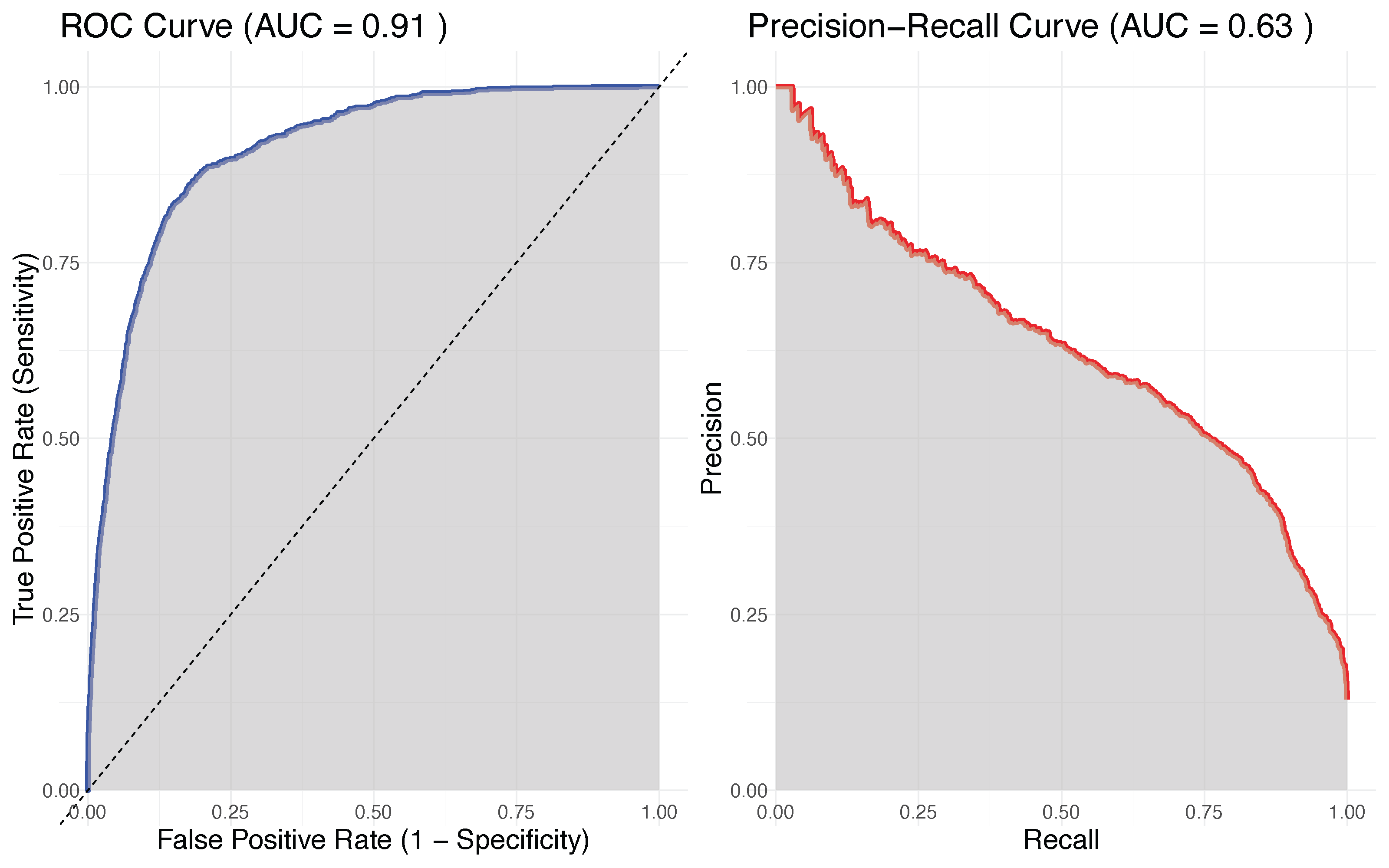
ROC curve and PR-AUC curve for RF classifier from esophageal study of adjuvant treatment versus surgery
Why does the classifier have such poor performance?
The problem here (and for other ML methods) is the equal misclassification costs used by the Bayes decision rule \[ \delta(\mathbf{x})=1 \hskip5pt\text{if}\hskip5pt P\{Y = 1 \mid \mathbf{X} = \mathbf{x}\} \ge \frac{1}{2} \]
In imbalanced data, the probability of an event is very small!! Therefore, the classifier tends to classify all cases as class labels 0
RFQ (random forest quantile) classifier
Use a different threshold. In place of 0.5 (the median) we use \(\pi=P\{Y=1\}\) \[ \delta(\mathbf{x})=1 \hskip5pt\text{if}\hskip5pt P\{Y = 1 \mid \mathbf{X} = \mathbf{x}\} \ge \pi \approx \frac{N_1}{N_0+N_1} \]
This has a dual optimality property (cost-weighted Bayes optimal and maximizes TNR+TPR)
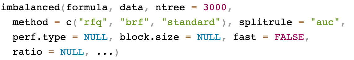
General call to imbalanced
Classification example: Glioma
Imbalanced class
Tip
imbalanced() is useful if you have two imbalanced class labels
data(glioma, package = "varPro")
table(glioma$y)
>     Classic-like            Codel      G-CIMP-high       G-CIMP-low         LGm6-GBM Mesenchymal-like          PA-like
>              148              174              249               25               41              215               26

## make a super majority class
class.combine <- c("Classic-like", "Codel", "G-CIMP-high", "Mesenchymal-like")
ynew <- factor(1 * !is.element(glioma$y, class.combine))

## replace y with the new super class
glioma2 <- glioma
glioma2$y <- ynew
table(glioma2$y)
>    0   1
>  786  94
Imbalanced classification: Glioma
standard RF classifier
## standard RF classifier
o1 <- rfsrc(y~.,glioma2)
print(o1)
                         Sample size: 880
           Frequency of class labels: 0=786, 1=94
                     Number of trees: 500
           Forest terminal node size: 1
       Average no. of terminal nodes: 29.802
No. of variables tried at each split: 36
              Total no. of variables: 1241
       Resampling used to grow trees: swor
    Resample size used to grow trees: 556
                            Analysis: RF-C
                              Family: class
                      Splitting rule: gini *random*
       Number of random split points: 10
                    Imbalanced ratio: 8.3617
                   (OOB) Brier score: 0.03485757
        (OOB) Normalized Brier score: 0.13943029
                           (OOB) AUC: 0.98882031
                      (OOB) Log-loss: 0.12614254
                        (OOB) PR-AUC: 0.92976788
                        (OOB) G-mean: 0.750886
   (OOB) Requested performance error: 0.04659091, 0, 0.43617021

Confusion matrix:

          predicted
  observed   0  1 class.error
         0 786  0      0.0000
         1  42 52      0.4468

      (OOB) Misclassification rate: 0.04772727

Random-classifier baselines (uniform):
   Brier: 0.25   Normalized Brier: 1   Log-loss: 0.69314718
Imbalanced classification: Glioma
RFQ classifier
## RFQ classifier
o2 <- imbalanced(y~.,glioma2)
print(o2)
                         Sample size: 880
           Frequency of class labels: 0=786, 1=94
                     Number of trees: 3000
           Forest terminal node size: 1
       Average no. of terminal nodes: 26.6797
No. of variables tried at each split: 36
              Total no. of variables: 1241
       Resampling used to grow trees: swor
    Resample size used to grow trees: 556
                            Analysis: RFQ
                              Family: class
                      Splitting rule: auc *random*
       Number of random split points: 10
                    Imbalanced ratio: 8.3617
                   (OOB) Brier score: 0.03394608
        (OOB) Normalized Brier score: 0.13578431
                           (OOB) AUC: 0.99057983
                      (OOB) Log-loss: 0.12099248
                        (OOB) PR-AUC: 0.94056031
                        (OOB) G-mean: 0.93762192
   (OOB) Requested performance error: 0.06237808

Confusion matrix:

          predicted
  observed   0  1 class.error
         0 691 95      0.1209
         1   0 94      0.0000

      (OOB) Misclassification rate: 0.1079545

Random-classifier baselines (uniform):
   Brier: 0.25   Normalized Brier: 1   Log-loss: 0.69314718
Imbalanced classification: Glioma
Balanced RF (BRF)
- BRF under-samples the majority class to balance the frequencies
- This is an example of a data-level method
- Surprisingly, BRF is actually an example of a quantile classifier and is theoretically equivalent to RFQ
- However, in finite samples it is less efficient
Imbalanced classification: Glioma
## BRF classifier
o3 <- imbalanced(y~.,glioma2, method = "brf")
print(o3)
                         Sample size: 880
           Frequency of class labels: 0=786, 1=94
                     Number of trees: 3000
           Forest terminal node size: 1
       Average no. of terminal nodes: 15.208
No. of variables tried at each split: 36
              Total no. of variables: 1241
       Resampling used to grow trees: swr
    Resample size used to grow trees: 188
                            Analysis: RF-C
                              Family: class
                      Splitting rule: auc *random*
       Number of random split points: 10
                    Imbalanced ratio: 8.3617
                   (OOB) Brier score: 0.04790004
        (OOB) Normalized Brier score: 0.19160015
                           (OOB) AUC: 0.9861269
                      (OOB) Log-loss: 0.1954276
                        (OOB) PR-AUC: 0.91991245
                        (OOB) G-mean: 0.91159495
   (OOB) Requested performance error: 0.08840505

Confusion matrix:

          predicted
  observed   0  1 class.error
         0 758 28      0.0356
         1  13 81      0.1383

      (OOB) Misclassification rate: 0.04659091

Random-classifier baselines (uniform):
   Brier: 0.25   Normalized Brier: 1   Log-loss: 0.69314718
Imbalanced classification: Glioma
## gmean variable importance with ci
o2 <- imbalanced(y~.,glioma2, importance="permute", block.size=20)
oo2 <- subsample(o2)
plot.subsample(oo2)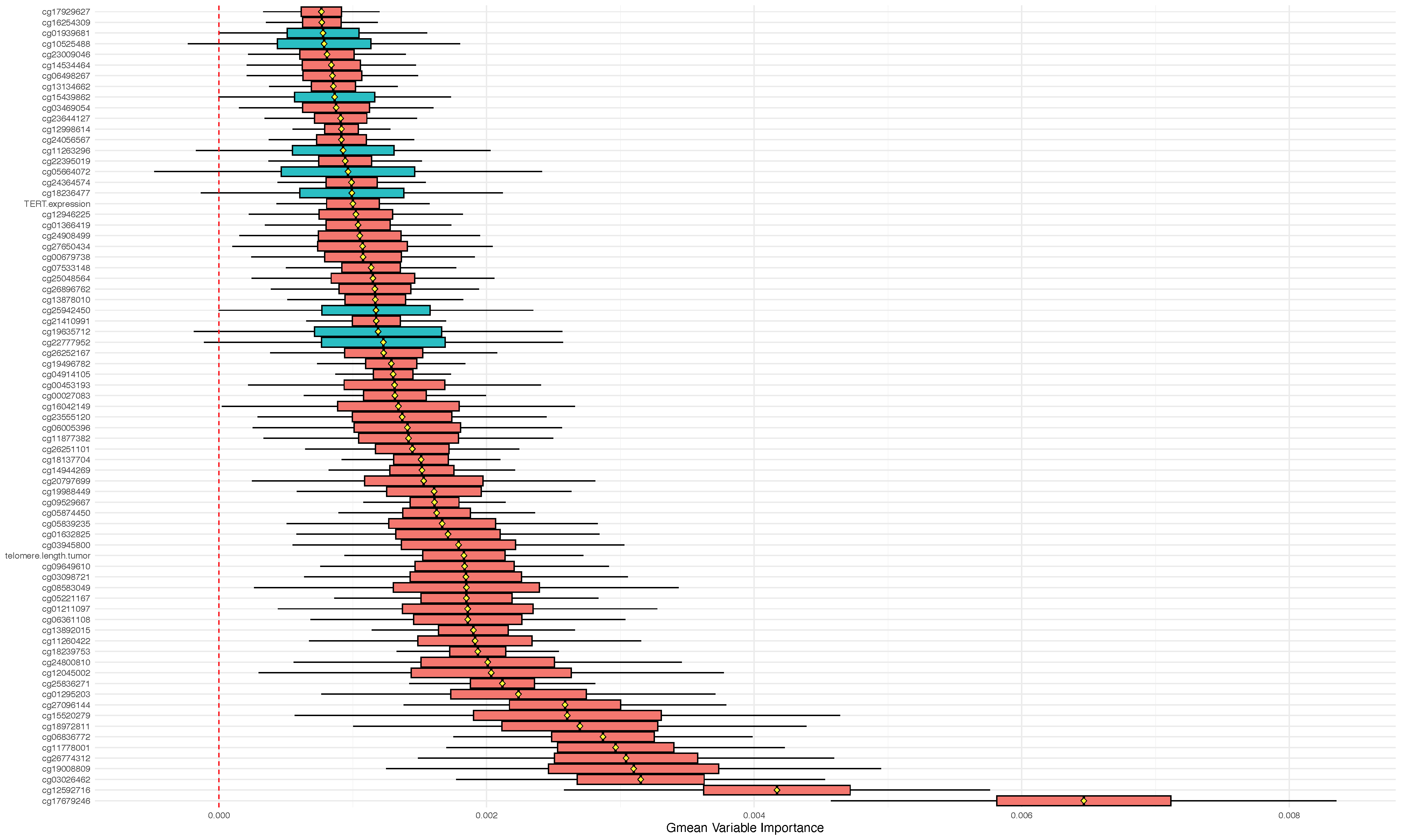
Competing risk
| Family | Example Grow Call with Formula Specification |
|---|---|
| Regression Quantile Regression |
rfsrc(Ozone~., data = airquality) quantreg(mpg~., data = mtcars)
|
|
Classification Imbalanced Two-Class |
rfsrc(Species~., data = iris) imbalanced(status~., data = breast)
|
| Survival | rfsrc(Surv(time, status)~., data = veteran) |
| Competing Risk | rfsrc(Surv(time, status)~., data = wihs) |
| Multivariate Regression Multivariate Mixed Regression Multivariate Quantile Regression Multivariate Mixed Quantile Regression |
rfsrc(Multivar(mpg, cyl)~., data = mtcars) rfsrc(cbind(Species,Sepal.Length)~.,data=iris) quantreg(cbind(mpg, cyl)~., data = mtcars) quantreg(cbind(Species,Sepal.Length)~.,data=iris)
|
| Unsupervised sidClustering Breiman (Shi-Horvath) |
rfsrc(data = mtcars) sidClustering(data = mtcars) sidClustering(data = mtcars, method = "sh")
|
Competing risk
This is a specialized survival (time to event) analysis setting:
- In competing risk the individual is subject to more than one event.
- For example, a patient listed to receive a heart transplant can die while on the waitlist, or they can receive the heart. The patient is subject to two competing risks “death” and “transplant”
- Right-censoring also occurs just like in standard survival analysis
Learn more [2]: https://www.randomforestsrc.org/articles/competing.html
Competing risk quantities of interest
There are two primary quantities of interest:
1. The cumulative incidence function (CIF) equal to the probability of observing an event of interest by time \(t\)
- Use the splitrule
logrankCR(the default) - Plot the values for
obj$cif - Use minimal depth for importance
2. The cause-specific hazard function equal to the instantaneous risk of event of interest \(j\) occuring at time \(t\)
- Use the splitrule
logrankand optioncause=j - Use option
importance='permute'to obtain importance and extract column \(j\) ofobj$importance
Competing risk example: PBC Mayo Clinic
Competing risk example: PBC Mayo Clinic
## canonical example: default Gray's splitting-rule
o <- rfsrc(Surv(time, status) ~ ., pbc)
o
                         Sample size: 276
                    Number of events: 1=18, 2=111
                     Number of trees: 500
           Forest terminal node size: 15
       Average no. of terminal nodes: 13.272
No. of variables tried at each split: 5
              Total no. of variables: 17
       Resampling used to grow trees: swor
    Resample size used to grow trees: 174
                            Analysis: RSF
                              Family: surv-CR
                      Splitting rule: logrankCR *random*
       Number of random split points: 10
   (OOB) Requested performance error: 0.19981499, 0.1685511
Tip
rfsrc recognize competing risk problem automatically when using the survival formula
event specific and non-event specific variable selection
## canonical example: default Gray's splitting-rule
## status: 0/1/2 for censored, transplant, dead
o <- rfsrc(Surv(time, status) ~ ., pbc)

## log-rank splitting where each event type is treated as the event of interest
## log-rank cause-1 specific splitting and targeted VIMP for cause 1="transplant"
o.log1 <- rfsrc(Surv(time, status) ~ ., pbc,
                splitrule = "logrank", cause = 1, importance = "permute")

## log-rank cause-2 specific splitting and targeted VIMP for cause 2="death"
o.log2 <- rfsrc(Surv(time, status) ~ ., pbc,
                splitrule = "logrank", cause = 2, importance = "permute")

## extract minimal depth from the Gray split forest: non-event specific
## extract VIMP from the log-rank forests: event-specific
var.perf <- data.frame(md = max.subtree(o)$order[, 1],
                       vimp1 = 100 * o.log1$importance[ ,1],
                       vimp2 = 100 * o.log2$importance[ ,2])
print(var.perf[order(var.perf$md), ], digits = 2)
          md  vimp1   vimp2
bili     2.0  6.407  5.9263
copper   3.5  2.944  2.0612
edema    4.3 -0.140  1.1829
albumin  4.3 -0.820  0.6809
ascites  4.5 -0.012  1.2883
protime  4.7 -0.832  0.5708
age      5.0  7.742  0.8564
chol     5.0  0.304  0.5097
ast      5.6 -0.345  0.3896
alk.phos 6.0 -1.068  0.0504
trig     6.0 -0.485  0.0089
stage    6.1  0.866  0.3493
platelet 6.3  0.409 -0.1191
hepato   6.6  0.772  0.1488
spiders  7.2 -0.121  0.1349
sex      7.3  0.125  0.0289
trt      7.9 -0.217 -0.0174
CIF stratified by edema
## cumulative incidence function (CIF) for transplant and dead stratified by edema
cif <- o$cif.oob; Time <- o$time.interest
edema <- o$xvar$edema
cif.transplant <- cbind(apply(cif[,,1][edema == 0,], 2, mean),
                        apply(cif[,,1][edema > 0,], 2, mean))
cif.dead  <- cbind(apply(cif[,,2][edema == 0,], 2, mean),
                   apply(cif[,,2][edema > 0,], 2, mean))
matplot(Time, cbind(cif.transplant, cif.dead), type = "l",
        lty = c(1,2,1,2), col = c(4, 4, 2, 2), lwd = 3, ylab = "CIF")
legend("topleft", legend = c("Transplant (No Edema)", "Transplant (Edema)",
                  "Dead (No Edema)", "Dead (Edema)"),
       lty = c(1,2,1,2), col = c(4, 4, 2, 2), lwd = 3, cex = 1.1)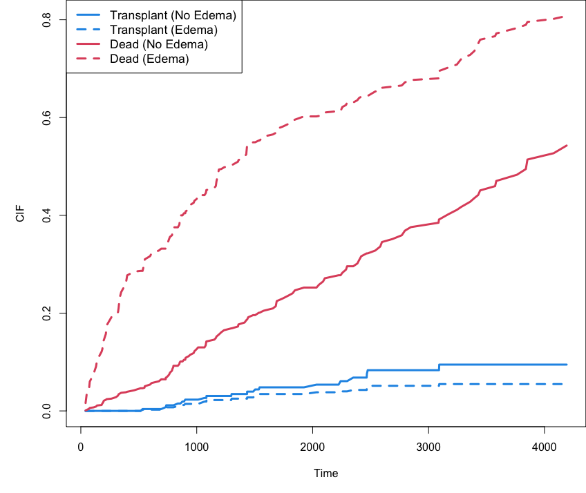
The run.rfsrc function for an overview
## tip!!! perform the same analysis as above with one line
run.rfsrc(Surv(time, status) ~ ., pbc, ntree=1000, alpha=.10)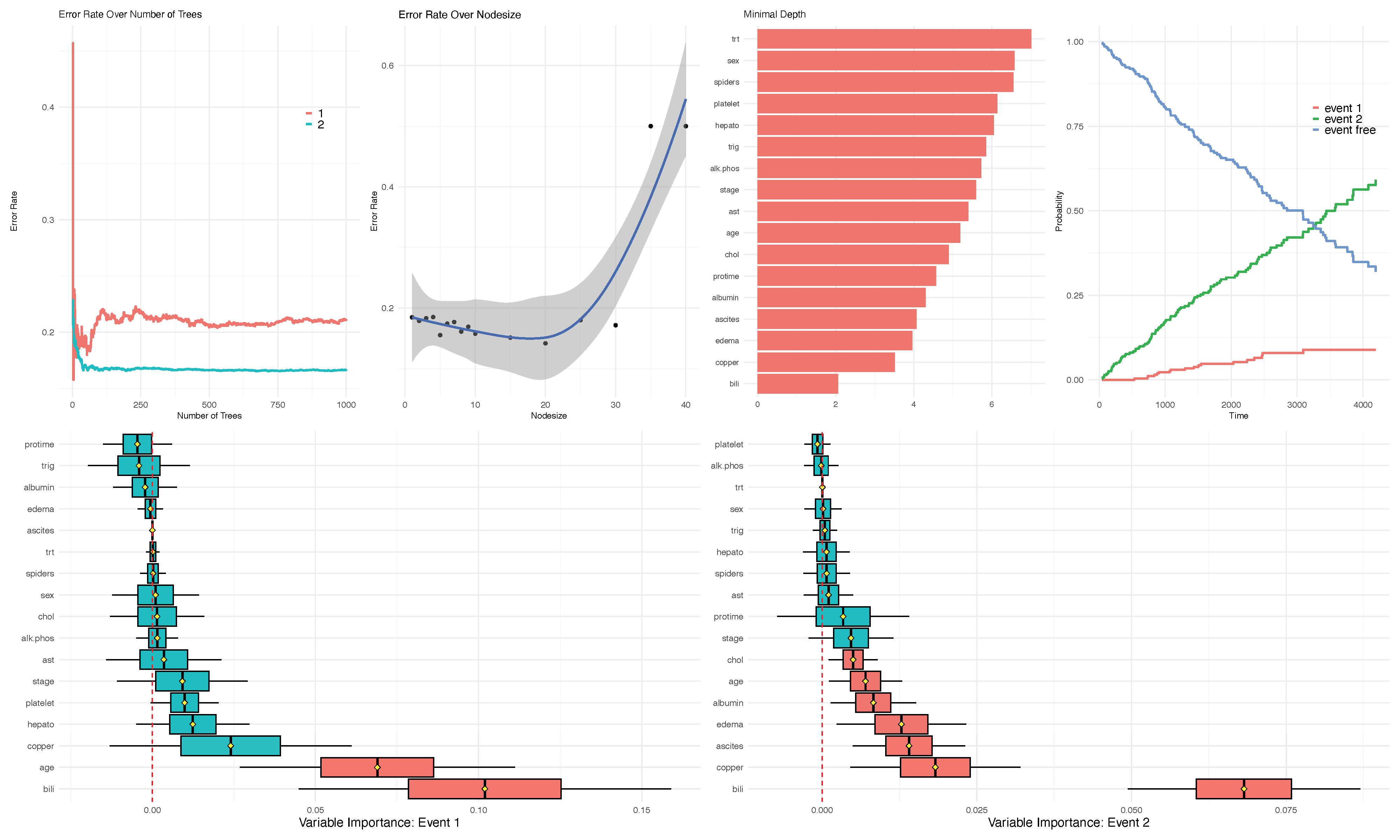
The run.rfsrc function for an overview
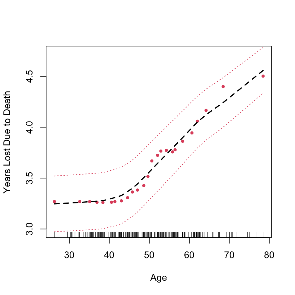
Partial plot
using “target” to specify the event of interest
pbc.cr$time <- pbc.cr$time/365
## target = an integer value between 1 and J indicating the event of interest
plot.variable(o.log1, target = 1,
              xvar.names = "age", partial = TRUE, smooth.lines = TRUE)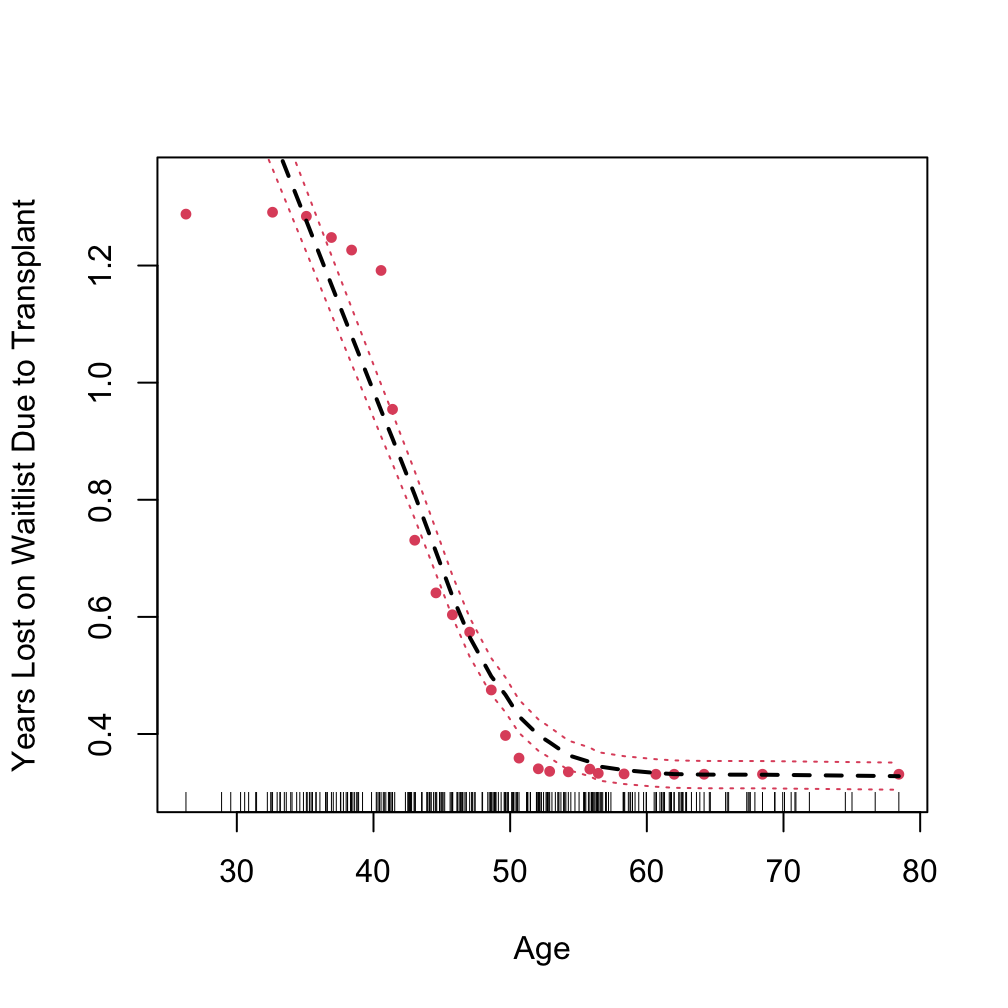
Partial plot
using “target” to specify the event of interest
Multivariate analysis
| Family | Example Grow Call with Formula Specification |
|---|---|
| Regression Quantile Regression |
rfsrc(Ozone~., data = airquality) quantreg(mpg~., data = mtcars)
|
|
Classification Imbalanced Two-Class |
rfsrc(Species~., data = iris) imbalanced(status~., data = breast)
|
| Survival | rfsrc(Surv(time, status)~., data = veteran) |
| Competing Risk | rfsrc(Surv(time, status)~., data = wihs) |
| Multivariate Regression Multivariate Mixed Regression Multivariate Quantile Regression Multivariate Mixed Quantile Regression |
rfsrc(Multivar(mpg, cyl)~., data = mtcars) rfsrc(cbind(Species,Sepal.Length)~.,data=iris) quantreg(cbind(mpg, cyl)~., data = mtcars) quantreg(cbind(Species,Sepal.Length)~.,data=iris)
|
| Unsupervised sidClustering Breiman (Shi-Horvath) |
rfsrc(data = mtcars) sidClustering(data = mtcars) sidClustering(data = mtcars, method = "sh")
|
Learn more [3]: https://www.randomforestsrc.org/articles/mvsplit.html
Multivariate example: Nutrigenomic Study
Study the effects of five diet treatments on 21 liver lipids and 120 hepatic gene expression in wild-type and PPAR-alpha deficient mice. We regress gene expression, diet and genotype (x-variables) on lipid expressions (multivariate y-responses) [4]
| C14.0 | C16.0 | C18.0 | C16.1n.9 | C16.1n.7 | C18.1n.9 | C18.1n.7 | diet | genotype | X36b4 | ACAT1 | ACAT2 | ACBP | ACC1 | ACC2 | ACOTH | ADISP | ADSS1 | ALDH3 |
|---|---|---|---|---|---|---|---|---|---|---|---|---|---|---|---|---|---|---|
| 0.34 | 26.45 | 10.22 | 0.35 | 3.10 | 16.98 | 2.41 | lin | wt | -0.42 | -0.65 | -0.84 | -0.34 | -1.29 | -1.13 | -0.93 | -0.98 | -1.19 | -0.68 |
| 0.38 | 24.04 | 9.93 | 0.55 | 2.54 | 20.07 | 3.92 | sun | wt | -0.44 | -0.68 | -0.91 | -0.32 | -1.23 | -1.06 | -0.99 | -0.97 | -1.00 | -0.62 |
| 0.36 | 23.70 | 8.96 | 0.55 | 2.65 | 22.89 | 3.96 | sun | wt | -0.48 | -0.74 | -1.10 | -0.46 | -1.30 | -1.09 | -1.06 | -1.08 | -1.18 | -0.75 |
| 0.22 | 25.48 | 8.14 | 0.49 | 2.82 | 21.92 | 2.52 | fish | wt | -0.45 | -0.69 | -0.65 | -0.41 | -1.26 | -1.09 | -0.93 | -1.02 | -1.07 | -0.71 |
| 0.37 | 24.80 | 9.63 | 0.46 | 2.85 | 21.38 | 2.96 | ref | wt | -0.42 | -0.71 | -0.54 | -0.38 | -1.21 | -0.89 | -1.00 | -0.95 | -1.08 | -0.76 |
Multivariate example: Nutrigenomic Study
## parse into y and x data
ydta <- nutrigenomic$lipids
xdta <- data.frame(nutrigenomic$genes,
                   diet = nutrigenomic$diet,
                   genotype = nutrigenomic$genotype)

## multivariate regression forest call
o <- rfsrc(get.mv.formula(colnames(ydta)),
            data.frame(ydta, xdta),
            importance=TRUE, nsplit = 10,
            splitrule = "mahalanobis")
> print(o)
Sample size: 40
Number of trees: 500
Forest terminal node size: 5
Average no. of terminal nodes: 4.774
No. of variables tried at each split: 41
Total no. of variables: 122
Resampling used to grow trees: swor
Resample size used to grow trees: 25
Analysis: mRF-R
Family: regr+
Splitting rule: mahalanobis *random*
Number of random split points: 10
(OOB) Requested performance error: 9.828, 0.554, 8.29, 4.695, 0.059, 7.816, 42.496, 9.231, 0.015, 0.434, 63.52, 0.765, 0.034, 0.158, 16.66, 0.058, 0.392, 30.194, 0.029, 4.556, 0.632, 15.793Multivariate example: Nutrigenomic Study
## acquire the error rate for each of the 21-coordinates
## standardize to allow for comparison across coordinates
serr <- get.mv.error(o, standardize = TRUE)
> serr
C14.0 C16.0 C18.0 C16.1n.9 C16.1n.7 C18.1n.9 C18.1n.7 C20.1n.9 C20.3n.9 C18.2n.6 C18.3n.6
0.8671651 0.6519146 0.6632005 0.7146180 0.8788133 0.7754928 0.8148566 0.7766450 0.8629866 0.8355279 0.9773675
C20.2n.6 C20.3n.6 C20.4n.6 C22.4n.6 C22.5n.6 C18.3n.3 C20.3n.3 C20.5n.3 C22.5n.3 C22.6n.3
0.8439182 0.7456620 0.8378708 0.8915473 0.8949931 0.9301005 0.9438823 0.6832386 0.8470016 0.5416053 > head(svimp)
C14.0 C16.0 C18.0 C16.1n.9 C16.1n.7 C18.1n.9 C18.1n.7 C20.1n.9 C20.3n.9 C18.2n.6 C18.3n.6
X36b4 -0.0011838300 -0.0011120623 -2.986438e-03 -0.0023431724 -0.001224286 -0.002843073 -0.0015607315 -0.0005896246 -0.0000214573 0.0004547212 -0.0006680341
ACAT1 -0.0046534735 0.0029068448 9.230050e-04 0.0022818757 -0.005663879 0.003297788 -0.0031493826 -0.0016189507 -0.0013414155 -0.0002053584 -0.0010019447
ACAT2 0.0136148438 0.0081002291 2.995972e-03 0.0111641579 0.008484230 0.021038781 0.0173969634 0.0055616191 0.0041388219 0.0072896355 -0.0005133367
ACBP 0.0036475488 0.0335889422 1.050479e-02 0.0046146024 0.003332181 0.001875450 0.0058926949 0.0127454125 0.0089004756 0.0127657144 -0.0004641915
ACC1 -0.0006048965 -0.0002409629 -2.053589e-03 -0.0008960043 -0.001153418 -0.001132043 -0.0006816805 0.0019148640 -0.0011168252 0.0005493523 -0.0003399971
ACC2 0.0091886014 -0.0029555916 2.252395e-05 0.0002228193 0.011012313 0.004644160 0.0098393504 -0.0004550441 0.0068958281 0.0056158617 0.0015149188
C20.2n.6 C20.3n.6 C20.4n.6 C22.4n.6 C22.5n.6 C18.3n.3 C20.3n.3 C20.5n.3 C22.5n.3 C22.6n.3
X36b4 -0.0008007217 -0.0002797032 -9.960998e-05 -0.0016751088 -0.0011467476 0.0012917637 0.0009019783 -0.001953023 -0.0028467311 -0.004910317
ACAT1 0.0016278408 0.0015450041 1.460450e-03 0.0039728775 -0.0002436180 -0.0015271289 -0.0009404719 0.002487745 0.0085764654 0.002279551
ACAT2 0.0163623835 0.0039925515 1.082762e-02 0.0243844140 0.0234540852 0.0256505212 0.0340391420 0.025389222 0.0117149395 0.010141345
ACBP 0.0054934515 0.0086732580 7.791429e-04 0.0015539132 -0.0023644673 0.0211272426 0.0095212814 0.005460451 0.0069928914 0.009941966
ACC1 -0.0003640483 -0.0024303740 -1.041940e-03 0.0000992922 -0.0004331203 -0.0008617263 -0.0009875129 -0.001643309 -0.0007186863 -0.003139676
ACC2 -0.0010663573 -0.0007101648 -1.196044e-03 -0.0014820461 -0.0023466329 0.0017062532 0.0006796071 0.002065533 -0.0011808523 0.003489718Split rules for multivariate regression
| Family | splitrule |
|---|---|
| Regression Quantile Regression |
mse la.quantile.regr, quantile.regr, mse
|
| Classification Imbalanced Two-Class |
gini, auc, entropy gini, auc, entropy
|
| Survival | logrank, bs.gradient, logrankscore |
| Competing Risk | logrankCR, logrank |
|
Multivariate Regression Multivariate Classification Multivariate Mixed Regression Multivariate Quantile Regression Multivariate Mixed Quantile Regression |
mv.mse, mahalanobis mv.gini mv.mix mv.mse mv.mix
|
| Unsupervised sidClustering Breiman (Shi-Horvath) |
unsupv \(\{\) mv.mse, mv.gini, mv.mix\(\}\), mahalanobis gini, auc, entropy
|
Split rules
mahalanobis splitting
o <- rfsrc(get.mv.formula(colnames(ydta)),
             data.frame(ydta, xdta),
             importance=TRUE, nsplit = 10,
             splitrule = "mahalanobis")
> print(o)
                         Sample size: 40
                     Number of trees: 500
           Forest terminal node size: 5
       Average no. of terminal nodes: 4.754
No. of variables tried at each split: 41
              Total no. of variables: 122
       Resampling used to grow trees: swor
    Resample size used to grow trees: 25
                            Analysis: mRF-R
                              Family: regr+
                      Splitting rule: mahalanobis *random*
       Number of random split points: 10
   (OOB) Requested performance error: 9.68, 0.553, 8.162, 4.763, 0.06, 7.737, 42.574, 9.289, 0.015, 0.442, 61.226, 0.766, 0.033, 0.156, 16.106, 0.054, 0.383, 30.393, 0.03, 4.733, 0.609, 15.203
Split rules
default composite (independence) splitting
o2 <- rfsrc(get.mv.formula(colnames(ydta)),
              data.frame(ydta, xdta),
              importance=TRUE, nsplit = 10)

> print(o2)
                         Sample size: 40
                     Number of trees: 500
           Forest terminal node size: 5
       Average no. of terminal nodes: 4.454
No. of variables tried at each split: 41
              Total no. of variables: 122
       Resampling used to grow trees: swor
    Resample size used to grow trees: 25
                            Analysis: mRF-R
                              Family: regr+
                      Splitting rule: mv *random*
       Number of random split points: 10
   (OOB) Requested performance error: 7.119, 0.387, 6.725, 3.527, 0.044, 5.519, 29.603, 5.488, 0.016, 0.28, 41.112, 0.757, 0.023, 0.101, 10.656, 0.036, 0.312, 27.217, 0.027, 3.551, 0.52, 13.606
Split rules
compare VIMP under the two split rules
## compare standardized VIMP for top 25 variables
imp <- data.frame(mahalanobis = rowMeans(get.mv.vimp(o,  standardize = TRUE)),
                  default     = rowMeans(get.mv.vimp(o2, standardize = TRUE)))
> print(100 * imp[order(imp[,"mahalanobis"], decreasing = TRUE)[1:25], ])
mahalanobis default
diet 10.1554383 50.157098614
CYP3A11 6.9094201 7.390394227
CYP2c29 4.3809975 2.318045460
PMDCI 3.0008368 4.127672741
Ntcp 2.2830390 1.219654570
genotype 2.0163456 7.149894438
CYP4A10 1.2867264 -0.032280665
SR.BI 1.2344900 1.298163431
GSTpi2 1.1666067 2.810511592
THIOL 1.0794705 1.230275963
CAR1 1.0716575 2.320816813
SPI1.1 0.9334952 1.622246274
G6Pase 0.8642624 0.121325455
Lpin 0.8477423 3.189846540
AOX 0.8048813 0.004006545
mHMGCoAS 0.7943659 0.419456736
FAT 0.7777474 -0.045086923
PLTP 0.5652898 1.217041153
ACOTH 0.5040769 1.326771272
Tpbeta 0.5003534 -0.054229018
L.FABP 0.4952051 -0.061771625
Tpalpha 0.4547016 0.221539122
ACBP 0.4307385 0.985221687
BSEP 0.4185126 0.248101073
FDFT 0.4046558 0.235316552The run.rfsrc function for an overview


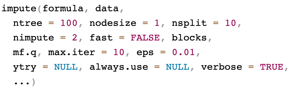
Missing data imputation
Missing data can be imputed at various stages of the analysis
- During training using
na.action="na.impute"inrfsrc - When predicting data using
na.action="na.impute"inpredict - Prior to any analysis using
impute
There are two methods used for imputing missing data
- OTFI (On the fly imputation): simultaneously impute data while growing a tree
- missForest: grow a forest using each variable as the \(y\) outcome and predicting the missing values
General call to impute
OTFI
- Only non-missing data are used for split-statistics. Daughter node membership assignment for missing data is made by sampling from the non-missing inbag data
- Can be used for supervised settings
- Also applicable to unsupervised settings. In this case multivariate splitting is applied to
ytryvariables which act as pseudo-responses
missForest and mForest
(multivariate missForest)
The imputation problem is turned into a series of regression problem
For datasets with a large number of variables, instead of running \(p\) regressions for each cycle, we can group variables into multivariate regressions
Ecosystem
RF-SRC — randomForestSRC
- Random Forests: classification, regression, survival (RSF & competing risks)
- OOB error, permutation VIMP, partial dependence/effect, proximities, imputation
- OpenMP compute backend
SGT — randomForestSGT
- Super Greedy Trees with multivariate geometric splits
- Currently emphasizes regression
VarPro — varPro
- Supervised model-independent variable selection (Variable Priority)
- Produces VI scores under supervision; complements permutation VIMP
RHF — randomForestRHF
- Random Hazard Forest for time-dependent hazard estimation
- Extends RSF to time-varying covariates
Statistical Families (Problem Types)
| Family | RF-SRC | VarPro | SGT | RHF |
|---|---|---|---|---|
| Binary / Multiclass Classification | Yes | Supervised VI for classification | Planned1 | Indirect (hazard focus) |
| Continuous Regression | Yes | Supervised VI for regression | Yes (primary) | Risk scores derived |
| Right-censored Survival (RSF) | Yes | Supervised VI for survival | Not primary | Yes (via hazard forest) |
| Competing Risks | Yes | Supervised VI | Not primary | Per-cause hazards2 |
| Time-varying Covariates | Limited (baseline RSF) | N/A | Not primary | Core capability |
| Unsupervised Feature Selection / VI | Heuristics (proximities) | UVarPro (unsupervised VI via release-based workflow) | Not core | Not core |
Outline
Part I: Training
- Quick start
- Data structures allowed
- Training (grow) with examples
(regression, classification, survival)
Part II: Inference and Prediction
- Inference (OOB)
- Prediction Error
- Prediction
- Restore
- Partial Plots
Part III: Variable Selection
- VIMP
- Subsampling (Confidence Intervals)
- Minimal Depth
- VarPro
Part IV: Advanced Examples
- Class Imbalanced Data
- Competing Risks
- Multivariate Forests
- Missing data imputation
References
1. Ishwaran H, O’Brien R, Lu M, Kogalur UB. randomForestSRC: Random forests quantile classifier (RFQ) vignette. 2021. http://randomforestsrc.org/articles/imbalance.html.
2. Ishwaran H, Gerds TA, Lau BM, Lu M, Kogalur UB. randomForestSRC: Competing risks vignette. 2021. http://randomforestsrc.org/articles/competing.html.
3. Ishwaran H, Tang F, Lu M, Kogalur UB. randomForestSRC: Multivariate splitting rule vignette. 2021. http://randomforestsrc.org/articles/mvsplit.html.
4. Martin PG, Guillou H, Lasserre F, Déjean S, Lan A, Pascussi J-M, et al. Novel aspects of PPAR\(\alpha\)-mediated regulation of lipid and xenobiotic metabolism revealed through a nutrigenomic study. Hepatology. 2007;45:767–77.
