Multiple Imputation for Missing Data in Meta-Analysis — metami • Computing Variances and Covariances, Visualization and Missing Data Solution for Multivariate Meta-Analysis with metavcov

Multiple imputation allows for the uncertainty about the missing data by generating several different plausible imputed data sets and appropriately combining results obtained from each of them. Let $\hat{\theta}_{*m}$ be the estimated coefficient from the $m$th imputed dataset for one of the $p$ dimensions in the multivariate outcome, where $m=1,\dots,M$. The coefficient from MI $\bar{\theta}$ is simply just an arithmetic mean of the individual coefficients estimated from each of the $M$ meta-analysis. We have $$\bar{\theta}=\frac{\sum_{m=1}^{M}\hat{\theta}_{*m}}{M}.$$ Estimation of the standard error for each variable is little more complicated. Let $V_W$ be the within imputation variance, which is the average of the variance of the estimated coefficient from each imputed dateset: $$V_W=\frac{\sum_{m=1}^{M}V ({\hat{\theta}_{*m}})}{M},$$ where $V ({\hat{\theta}_{*m}})$ is the variance of the estimator calculated from generalized least squares methods using the imputed dataset. Let $V_B$ be the between imputation variance, which is calculated as $$V_B=\frac{\sum_{m=1}^{M}({\hat{\theta}_{*m}}-\bar{\theta})^2}{M-1}.$$ From $V_W$ and $V_B$, the variance of the pooled coefficients is calculated as $$V(\bar{\theta})=V_W+V_B+\frac{V_B}{M}$$ The above variance is statistically principled since $V_W$ reflects the sampling variance and $V_B$ reflects the extra variance due to the missing data.

metami(data, M = 20, vcov = "r.vcov",
        r.n.name, ef.name, x.name = NULL,
        rvcov.method = "average", rvcov.zscore = TRUE,
        type = NULL,
        d = NULL, sdt = NULL, sdc = NULL,
        nt = NULL, nc = NULL,
        st = NULL, sc = NULL,
        n_rt = NA, n_rc = NA,
        r = NULL,
        func = "mvmeta",
        formula = NULL,
        method = "fixed",
        pool.seq = NULL,
        return.mi = FALSE,
        ci.level = 0.95)

Arguments

data	A $N \times p$ data frame that contains effect sizes and predictors for meta-regression, if any.
M	Number of imputed data sets.
vcov	Method for computing effect sizes; options including `vcov = "r.vcov"` for correlation coefficients and `vcov = "mix.vcov"` for other types of effect sizes. See `r.vcov` and `mix.vcov` for details.
r.n.name	A string defining the column name for sample sizes in `data` when the effect sizes are correlation coefficients (`vcov = "r.vcov"`).
ef.name	A $p$-dimensional vector that stores the column names for sample sizes in `data` when the effect sizes are correlation coefficients (`vcov = "r.vcov"`).
x.name	A vector that stores the column names in `data` for predictors for meta-regression.
rvcov.method	Method used for `r.vcov`; options including `"average"` and `"each"`.
rvcov.zscore	Whether the correlation coefficients in `data` are already transformed into Fisher's $z$ scores.
type	A $p$-dimensional vector indicating types of effect sizes for the argument `vcov = "mix.vcov"`. `"MD"` stands for mean difference, `"SMD"` stands for standardized mean difference, `"logOR"` stands for log odds ratio, `"logRR"` stands for log risk ratio, and `"RD"` stands for risk difference.
d	A $p$-dimensional vector that stores the column names in `data` for continuous effect sizes such as MD or SMD. If outcome $j$ is dichotomous, NA has to be imputed in for $d[j]$.
sdt	A $p$-dimensional vector that stores the column names in `data` for the sample standard deviations of each outcome from the treatment group. If outcome $j$ is dichotomous, NA has to be imputed in for $d[j]$.
sdc	A vector defined in a similar way as `sdt` for the control group.
nt	A $p$-dimensional vector that stores the column names in `data` for sample sizes of $p$ outcomes from treatment group.
nc	A vector defined in a similar way as `nt` for the control group.
st	A $p$-dimensional vector that stores the column names in `data` for the number of participants with event for all outcomes (dichotomous) in the treatment group. If outcome $j$ is dichotomous, NA has to be imputed in for $st[j]$.
sc	A vector defined in a similar way as `st` for the control group.
n_rt	A $N$-dimensional list of $p \times p$ correlation matrices storing sample sizes in the treatment group reporting pairwise outcomes in the off-diagonal elements. See `mix.vcov` for details.
n_rc	A list defined in a similar way as `n_rt` for the control group.
r	A $N$-dimensional list of $p \times p$ correlation matrices for the $p$ outcomes from the $N$ studies. See `mix.vcov` for details.
func	A string defining the function to be used for fitting the meta-analysis. Options include `func = "metafixed"` for fixed-effect meta-analysis (see `metafixed` for details). `func = "mvmeta"`, for which the `mvmeta` package must be installed beforehand, and `func = "meta"`, for which the `metaSEM` package must be installed beforehand.
formula	Formula used for the function `func = "mvmeta"` from the `mvmeta` package when `func = "mvmeta"`.
method	Method used for the function `func = "mvmeta"` from the `mvmeta` package when `func = "mvmeta"`.
pool.seq	A numeric vector indicating if the results are pooled from subsets of the `M` data sets. By default, the results are only pooled from all `M` data sets.
return.mi	Should the `M` imputed data sets be returned?
ci.level	Significant level for the pooled confidence intervals. The default is 0.05.

Author

Min Lu

Details

For the imputation phase, this function imports the mice package that imputes incomplete multivariate data by chained equations. The pooling phase is performed via the Rubin's rules.

Value

coefficients

A data.frame that contains the pooled results from the M imputed data sets.

results.mi

A $M$-dimensional list of results from each imputed data set.

data.mi

A $M$-dimensional list of imputed data sets if the argument return.mi = TRUE.

result.seq

A list of results from the pooled results from the subsets of the M imputed data sets if the argument pool.seq = TRUE.

References

Ahn, S., Lu, M., Lefevor, G.T., Fedewa, A. & Celimli, S. (2016). Application of meta-analysis in sport and exercise science. In N. Ntoumanis, & N. Myers (Eds.), An Introduction to Intermediate and Advanced Statistical Analyses for Sport and Exercise Scientists (pp.233-253). Hoboken, NJ: John Wiley and Sons, Ltd.

Cooper, H., Hedges, L.V., & Valentine, J.C. (Eds.) (2009). The handbook of research synthesis and meta-analysis. New York: Russell Sage Foundation.

Olkin, I., & Ishii, G. (1976). Asymptotic distribution of functions of a correlation matrix. In S. Ikeda (Ed.), Essays in probability and statistics: A volume in honor of Professor Junjiro Ogawa (pp.5-51). Tokyo, Japan: Shinko Tsusho.

Van Buuren, S. and Groothuis-Oudshoorn, K., 2011. mice: Multivariate imputation by chained equations in R. Journal of statistical software, 45(1), pp.1-67.

Gasparrini A., Armstrong, B., Kenward M. G. (2012). Multivariate meta-analysis for non-linear and other multi-parameter associations. Statistics in Medicine. 31(29):3821-3839.

Cheung, M.W.L. (2015). metaSEM: An R Package for Meta-Analysis using Structural Equation Modeling. Frontiers in Psychology 5, 1521.

Rubin, D.B., 2004. Multiple imputation for nonresponse in surveys (Vol. 81). John Wiley & Sons.

Examples

#####################################################################################
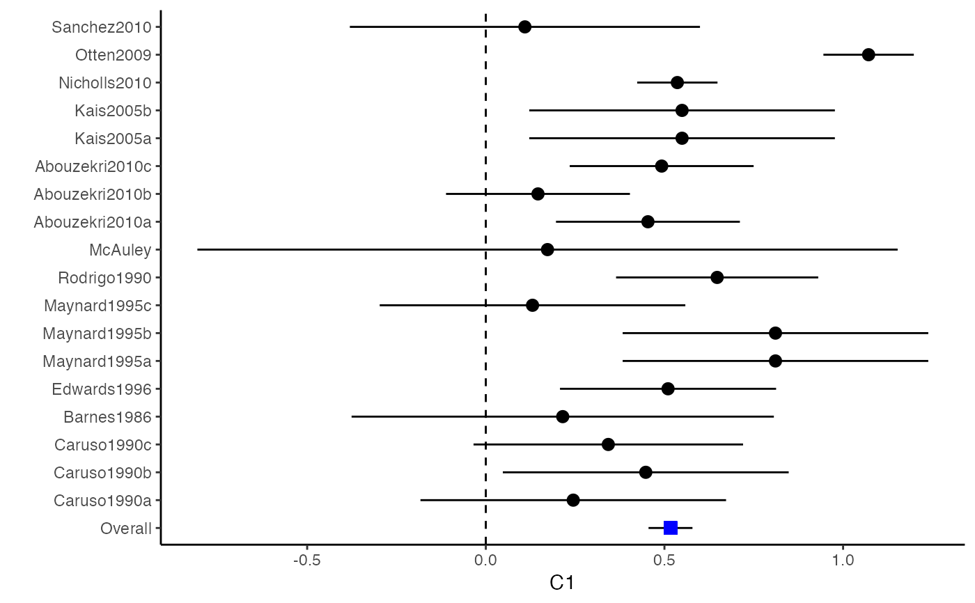
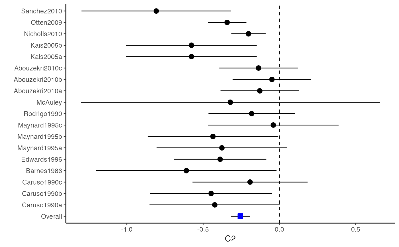
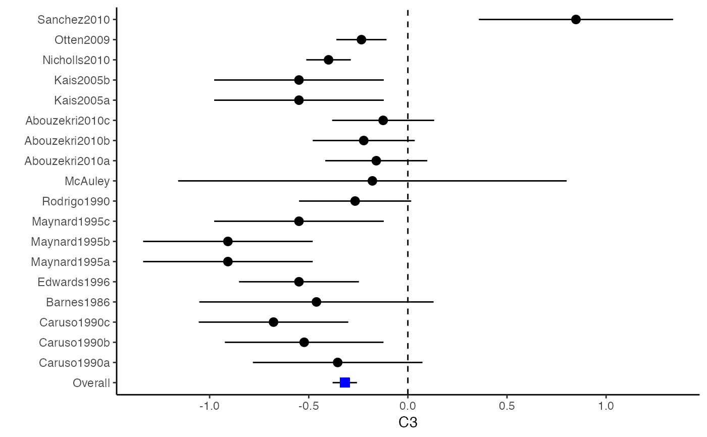
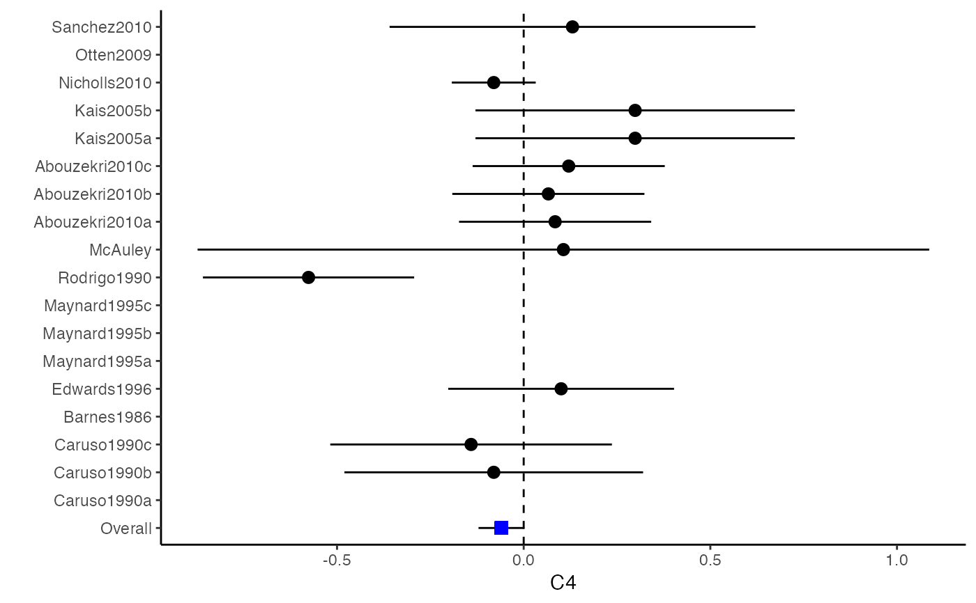
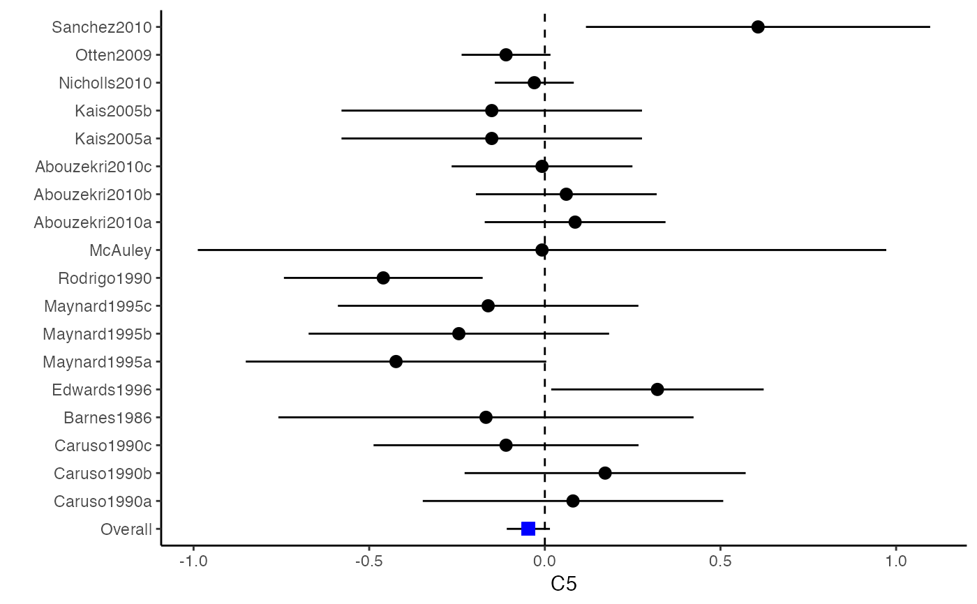
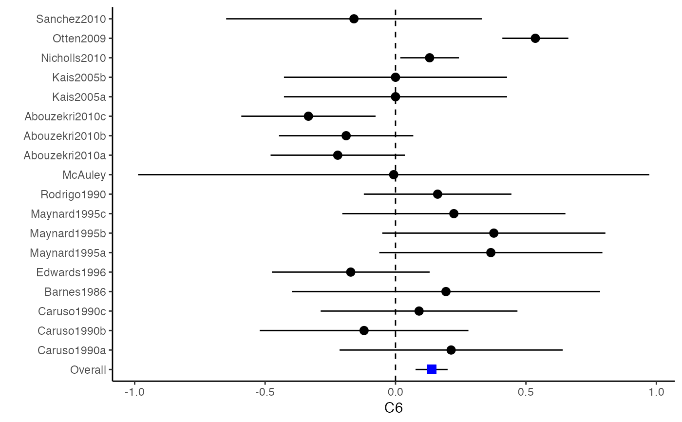
# Example: Craft2003 data
# Preparing input arguments for meta.mi() and fixed-effect model
#####################################################################################
# prepare a dataset with missing values and input arguments for meta.mi
Craft2003.mnar <- Craft2003[, c(2, 4:10)]
Craft2003.mnar[sample(which(Craft2003$C4 < 0), 6), "C4"] <- NA
dat <- Craft2003.mnar
n.name <- "N"
ef.name <- c("C1", "C2", "C3", "C4", "C5", "C6")
# fixed-effect model
obj <- metami(dat, M = 10, vcov = "r.vcov",
             n.name, ef.name,
             func = "metafixed")
#> pooled results from 10 imputations for missing values in C4 
#> Fixed-effects coefficients
#>     Estimate  Std. Error         z  Pr(>|z|)  95%ci.lb  95%ci.ub     
#> C1    0.5169      0.0314   16.4814    0.0000    0.4555    0.5784  ***
#> C2   -0.2558      0.0314   -8.1561    0.0000   -0.3172   -0.1943  ***
#> C3   -0.3182      0.0314  -10.1467    0.0000   -0.3796   -0.2567  ***
#> C4   -0.0596      0.0314   -1.9004    0.0574   -0.1211    0.0019    .
#> C5   -0.0469      0.0314   -1.4971    0.1344   -0.1084    0.0145     
#> C6    0.1382      0.0314    4.4072    0.0000    0.0768    0.1997  ***
#> ---
#> Signif. codes:  0 ‘***’ 0.001 ‘**’ 0.01 ‘*’ 0.05 ‘.’ 0.1 ‘ ’ 1 
#> 

########################
# Plotting the result
########################
computvcov <- r.vcov(n = Craft2003$N,
                     corflat = subset(Craft2003.mnar, select = C1:C6),
                     method = "average")
plotCI(y = computvcov$ef, v = computvcov$list.vcov,
        name.y = NULL, name.study = Craft2003$ID,
        y.all = obj$coefficients[,1],
        y.all.se = obj$coefficients[,2])
#> $`Plotting C1`
#> 
#> $`Plotting C2`
#> 
#> $`Plotting C3`
#> 
#> $`Plotting C4`
#> Warning: Removed 6 rows containing missing values (geom_pointrange).
#> 
#> $`Plotting C5`
#> 
#> $`Plotting C6`
#> 

########################
# Pooling from subsets
########################
o1 <- metami(dat, M = 10, vcov = "r.vcov",
              n.name, ef.name,
              func = "metafixed",
              pool.seq = c(5, 10))
#> pooled results from 10 imputations for missing values in C4 
#> Fixed-effects coefficients
#>     Estimate  Std. Error         z  Pr(>|z|)  95%ci.lb  95%ci.ub     
#> C1    0.5170      0.0314   16.4825    0.0000    0.4555    0.5784  ***
#> C2   -0.2560      0.0314   -8.1642    0.0000   -0.3175   -0.1945  ***
#> C3   -0.3182      0.0314  -10.1458    0.0000   -0.3796   -0.2567  ***
#> C4   -0.0501      0.0314   -1.5976    0.1101   -0.1116    0.0114     
#> C5   -0.0470      0.0314   -1.4998    0.1337   -0.1085    0.0144     
#> C6    0.1382      0.0314    4.4058    0.0000    0.0767    0.1997  ***
#> ---
#> Signif. codes:  0 ‘***’ 0.001 ‘**’ 0.01 ‘*’ 0.05 ‘.’ 0.1 ‘ ’ 1 
#> 
# pooled results from M = 5 imputed data sets
o1$result.seq$M5$coefficients
#>       Estimate Std. Error           z     Pr(>|z|)    95%ci.lb    95%ci.ub
#> C1  0.51683598 0.03136417  16.4785456 0.000000e+00  0.45536333  0.57830863
#> C2 -0.25631789 0.03135624  -8.1743812 2.220446e-16 -0.31777500 -0.19486078
#> C3 -0.31804815 0.03135804 -10.1424747 0.000000e+00 -0.37950878 -0.25658751
#> C4 -0.01607465 0.03135730  -0.5126286 6.082112e-01 -0.07753384  0.04538454
#> C5 -0.04727197 0.03135605  -1.5075871 1.316602e-01 -0.10872869  0.01418475
#> C6  0.13815009 0.03136602   4.4044512 1.060520e-05  0.07667382  0.19962635
# pooled results from M = 10 imputed data sets
o1$result.seq$M10$coefficients
#>       Estimate Std. Error          z     Pr(>|z|)    95%ci.lb    95%ci.ub
#> C1  0.51696741 0.03136463  16.482497 0.000000e+00  0.45549387  0.57844096
#> C2 -0.25600261 0.03135676  -8.164193 2.220446e-16 -0.31746073 -0.19454450
#> C3 -0.31815427 0.03135835 -10.145761 0.000000e+00 -0.37961549 -0.25669304
#> C4 -0.05009895 0.03135803  -1.597643 1.101224e-01 -0.11155955  0.01136166
#> C5 -0.04702938 0.03135615  -1.499845 1.336544e-01 -0.10848629  0.01442754
#> C6  0.13819176 0.03136610   4.405768 1.054095e-05  0.07671534  0.19966818
#########################################################################################
# Running random-effects and meta-regression model using packages "mvmeta" or "metaSEM"
#########################################################################################
# Restricted maximum likelihood (REML) estimator from the mvmeta package
# library(mvmeta)
# o2 <- metami(dat, M = 10, vcov = "r.vcov",
#                     n.name, ef.name,
#                     formula = as.formula(cbind(C1, C2, C3, C4, C5, C6) ~ . ),
#                     func = "mvmeta",
#                     method = "reml")
# maximum likelihood estimators from the metaSEM package
# library(metaSEM)
# o3 <- metami(dat, M = 10, vcov = "r.vcov",
#               n.name, ef.name,
#               func = "meta")

# meta-regression
# library(metaSEM)
# o4 <- metami(dat, M = 10, vcov = "r.vcov",
#                     n.name, ef.name, x.name = "p_male",
#                     func = "meta")
# library(mvmeta)
# o5 <- metami(dat, M = 20, vcov = "r.vcov",
#               n.name, ef.name, x.name = "p_male",
#               formula = as.formula(cbind(C1, C2, C3, C4, C5, C6) ~ p_male ),
#               func = "mvmeta",
#               method = "reml")
#####################################################################################
# Example: Geeganage2010 data
# Preparing input arguments for meta.mi() and fixed-effect model
#####################################################################################
# Geeganage2010.mnar <- Geeganage2010
# Geeganage2010.mnar$MD_SBP[sample(1:nrow(Geeganage2010),7)] <- NA
# r12 <- 0.71
# r13 <- 0.5
# r14 <- 0.25
# r23 <- 0.6
# r24 <- 0.16
# r34 <- 0.16
# r <- vecTosm(c(r12, r13, r14, r23, r24, r34))
# diag(r) <- 1
# mix.r <- lapply(1:nrow(Geeganage2010), function(i){r})
# o <- metami(data = Geeganage2010.mnar, M = 10, vcov = "mix.vcov",
#               ef.name = c("MD_SBP", "MD_DBP", "RD_DD", "lgOR_D"),
#               type = c("MD", "MD", "RD", "lgOR"),
#               d = c("MD_SBP", "MD_DBP", NA, NA),
#               sdt = c("sdt_SBP", "sdt_DBP", NA, NA),
#               sdc = c("sdc_SBP", "sdc_DBP", NA, NA),
#               nt = c("nt_SBP", "nt_DBP", "nt_DD", "nt_D"),
#               nc = c("nc_SBP", "nc_DBP", "nc_DD", "nc_D"),
#               st = c(NA, NA, "st_DD", "st_D"),
#               sc = c(NA, NA, "sc_DD", "sc_D"),
#               r = mix.r,
#               func = "metafixed")

data	A \(N \times p\) data frame that contains effect sizes and predictors for meta-regression, if any.
M	Number of imputed data sets.
vcov	Method for computing effect sizes; options including `vcov = "r.vcov"` for correlation coefficients and `vcov = "mix.vcov"` for other types of effect sizes. See `r.vcov` and `mix.vcov` for details.
r.n.name	A string defining the column name for sample sizes in `data` when the effect sizes are correlation coefficients (`vcov = "r.vcov"`).
ef.name	A \(p\)-dimensional vector that stores the column names for sample sizes in `data` when the effect sizes are correlation coefficients (`vcov = "r.vcov"`).
x.name	A vector that stores the column names in `data` for predictors for meta-regression.
rvcov.method	Method used for `r.vcov`; options including `"average"` and `"each"`.
rvcov.zscore	Whether the correlation coefficients in `data` are already transformed into Fisher's \(z\) scores.
type	A \(p\)-dimensional vector indicating types of effect sizes for the argument `vcov = "mix.vcov"`. `"MD"` stands for mean difference, `"SMD"` stands for standardized mean difference, `"logOR"` stands for log odds ratio, `"logRR"` stands for log risk ratio, and `"RD"` stands for risk difference.
d	A \(p\)-dimensional vector that stores the column names in `data` for continuous effect sizes such as MD or SMD. If outcome \(j\) is dichotomous, NA has to be imputed in for \(d[j]\).
sdt	A \(p\)-dimensional vector that stores the column names in `data` for the sample standard deviations of each outcome from the treatment group. If outcome \(j\) is dichotomous, NA has to be imputed in for \(d[j]\).
sdc	A vector defined in a similar way as `sdt` for the control group.
nt	A \(p\)-dimensional vector that stores the column names in `data` for sample sizes of \(p\) outcomes from treatment group.
nc	A vector defined in a similar way as `nt` for the control group.
st	A \(p\)-dimensional vector that stores the column names in `data` for the number of participants with event for all outcomes (dichotomous) in the treatment group. If outcome \(j\) is dichotomous, NA has to be imputed in for \(st[j]\).
sc	A vector defined in a similar way as `st` for the control group.
n_rt	A \(N\)-dimensional list of \(p \times p\) correlation matrices storing sample sizes in the treatment group reporting pairwise outcomes in the off-diagonal elements. See `mix.vcov` for details.
n_rc	A list defined in a similar way as `n_rt` for the control group.
r	A \(N\)-dimensional list of \(p \times p\) correlation matrices for the \(p\) outcomes from the \(N\) studies. See `mix.vcov` for details.
func	A string defining the function to be used for fitting the meta-analysis. Options include `func = "metafixed"` for fixed-effect meta-analysis (see `metafixed` for details). `func = "mvmeta"`, for which the `mvmeta` package must be installed beforehand, and `func = "meta"`, for which the `metaSEM` package must be installed beforehand.
formula	Formula used for the function `func = "mvmeta"` from the `mvmeta` package when `func = "mvmeta"`.
method	Method used for the function `func = "mvmeta"` from the `mvmeta` package when `func = "mvmeta"`.
pool.seq	A numeric vector indicating if the results are pooled from subsets of the `M` data sets. By default, the results are only pooled from all `M` data sets.
return.mi	Should the `M` imputed data sets be returned?
ci.level	Significant level for the pooled confidence intervals. The default is 0.05.