Computing Variances and Covariances, Visualization and Missing Data Solution for Multivariate Meta Analysis
metavcov-package.RdThe package metavcov computes variances and covariances for effect sizes as preparations for multivariate meta-analysis. Effect sizes include correlation (r), mean difference (MD), standardized mean difference (SMD), log odds ratio (logOR), log risk ratio (logRR), and risk difference (RD). Functions for plotting confidence intervals and multiple imputation for missing data are offered. It can fit a fixed-effect model for demonstration purposes; users are highly encouraged to use packages mvmeta and metaSEM for random-effect models.
Author
Min Lu (Maintainer,<m.lu6@umiami.edu>)
References
Ahn, S., Lu, M., Lefevor, G.T., Fedewa, A. & Celimli, S. (2016). Application of meta-analysis in sport and exercise science. In N. Ntoumanis, & N. Myers (Eds.), An Introduction to Intermediate and Advanced Statistical Analyses for Sport and Exercise Scientists (pp.233-253). Hoboken, NJ: John Wiley and Sons, Ltd.
Olkin, I., & Ishii, G. (1976). Asymptotic distribution of functions of a correlation matrix. In S. Ikeda (Ed.), Essays in probability and statistics: A volume in honor of Professor Junjiro Ogawa (pp.5-51). Tokyo, Japan: Shinko Tsusho.
B. J. Becker. (2009) Model-based meta-analysis. In H. Cooper, L. V. Hedges, and J. C. Valentine, (Ed.), The handbook of research synthesis and meta-analysis, chapter 20, pages 377-395. Russell Sage Foundation,
Wei, Y., & Higgins, J. (2013). Estimating within study covariances in multivariate meta-analysis with multiple outcomes. Statistics in Medicine, 32(7), 119-1205.
Examples
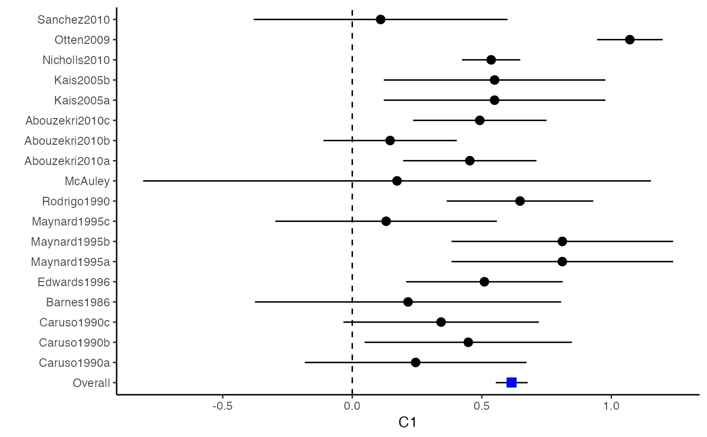
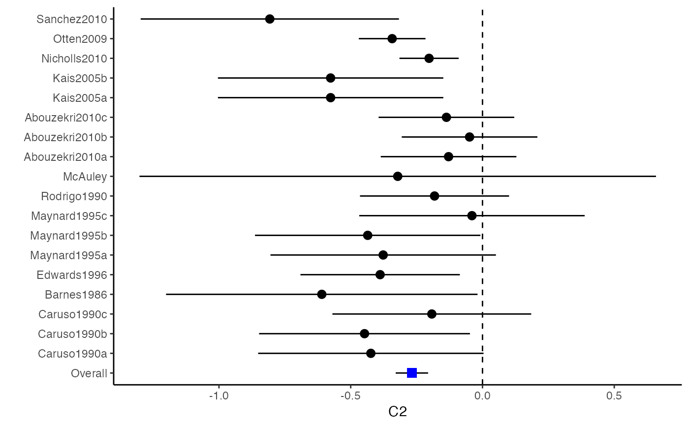
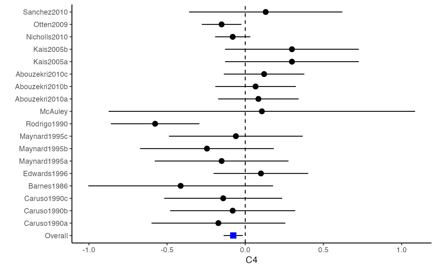
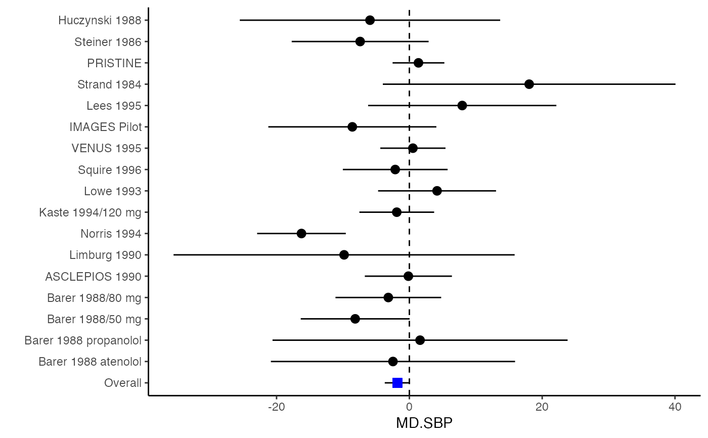
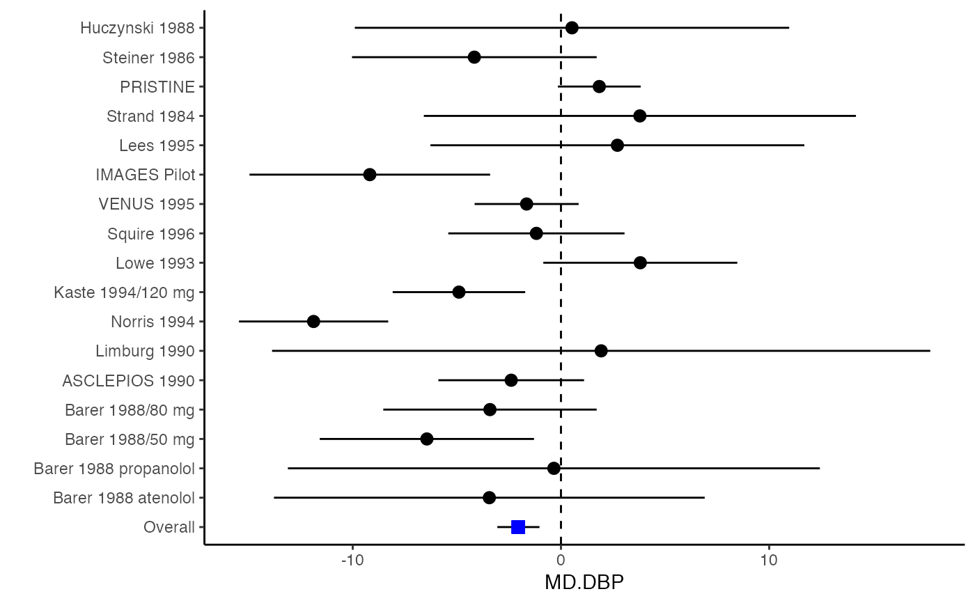
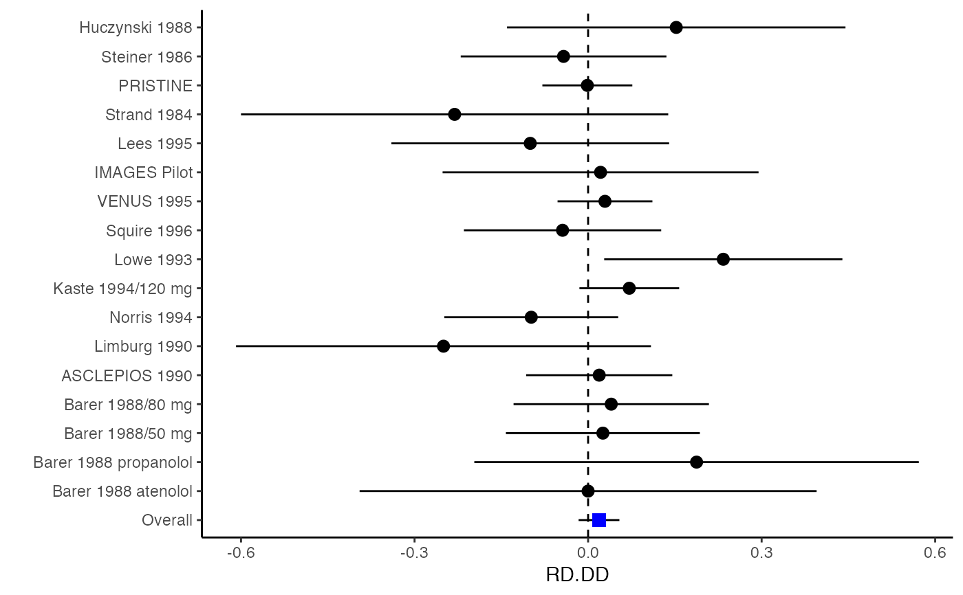
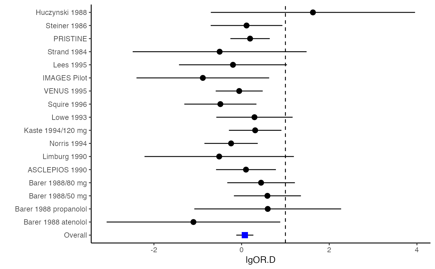
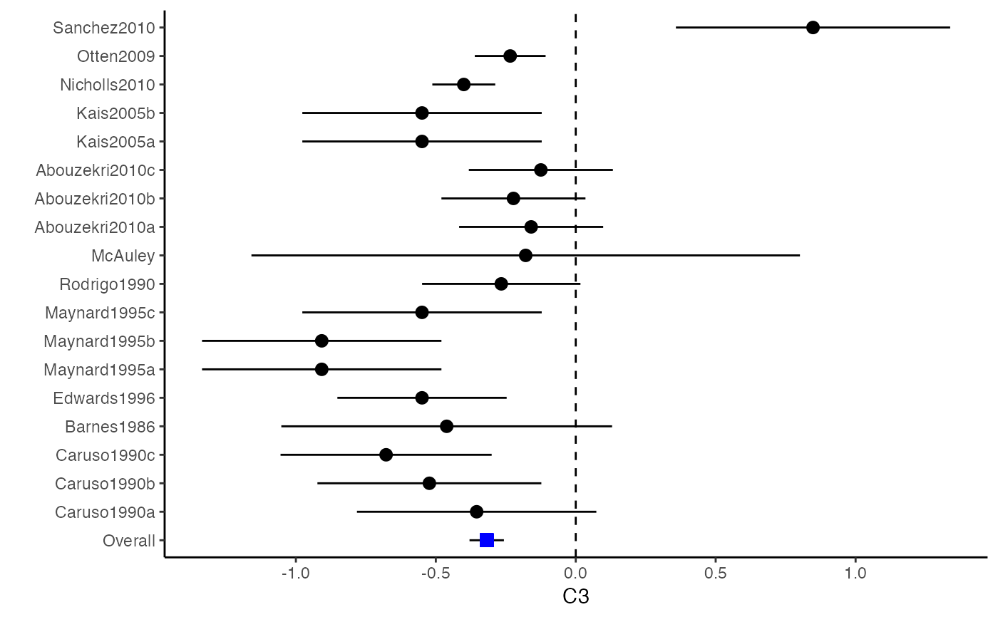
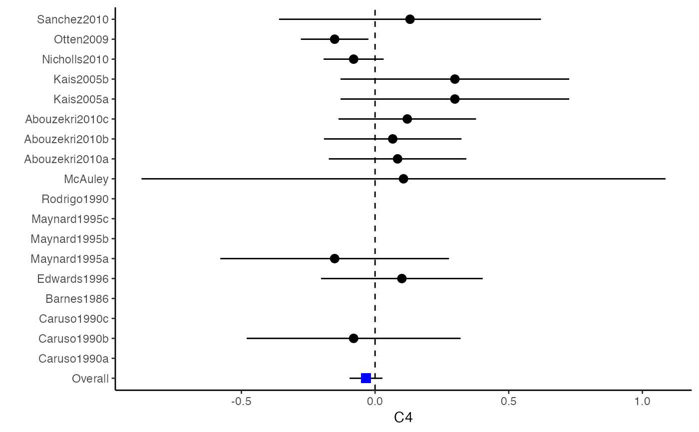
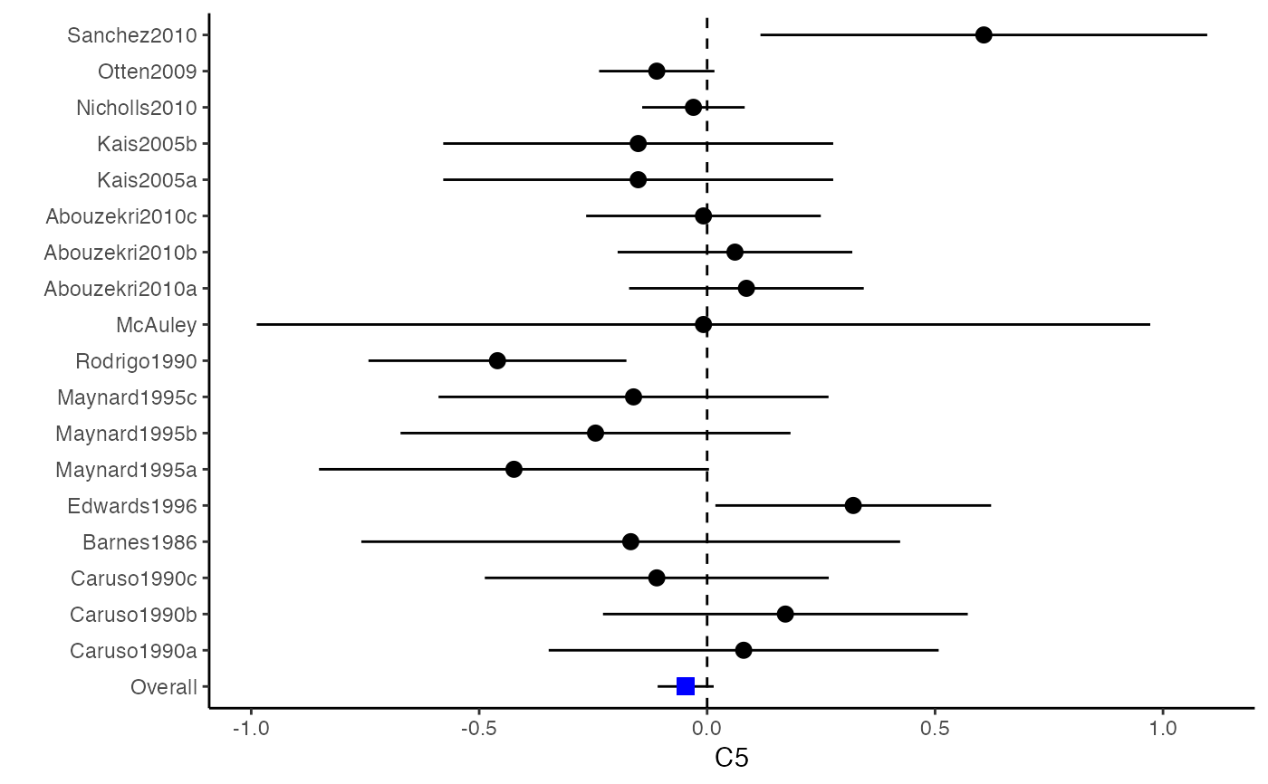
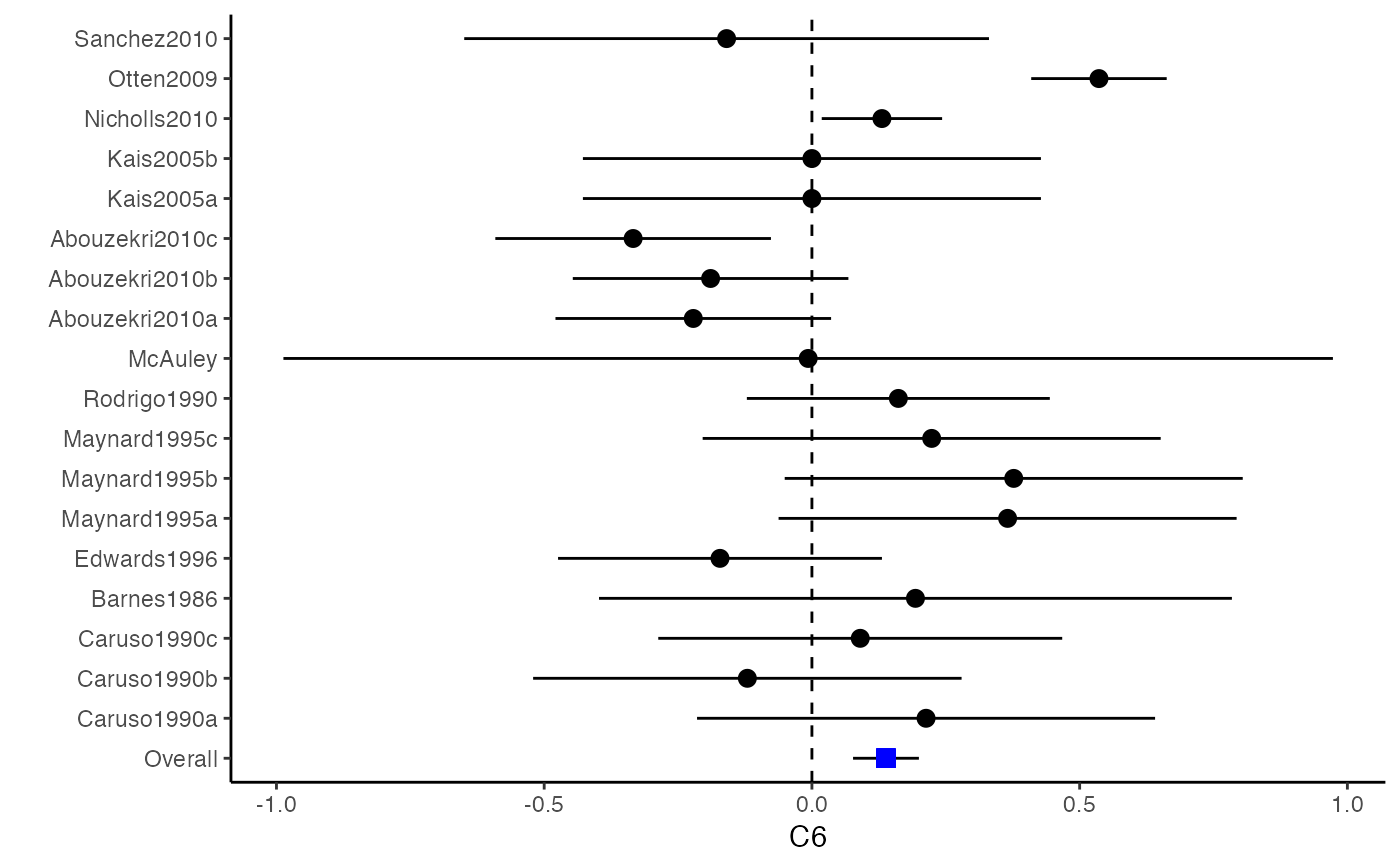
############################################### # Effect size: correlation coefficients ############################################### data(Craft2003) # extract correlation from the dataset (craft) corflat <- subset(Craft2003, select=C1:C6) # transform correlations to z and compute variance-covariance matrix. computvcov <- r.vcov(n = Craft2003$N, corflat = corflat, method = "average") # name transformed z scores as y y <- computvcov$ef # name variance-covariance matrix of trnasformed z scores as S S <- computvcov$matrix.vcov S[1, ]#> var_C1 cov_C1_C2 cov_C1_C3 cov_C1_C4 cov_C1_C5 #> 0.0476190476 -0.0001899941 0.0013681072 -0.0101984824 -0.0128884805 #> cov_C1_C6 var_C2 cov_C2_C3 cov_C2_C4 cov_C2_C5 #> -0.0004515741 0.0476190476 0.0037735402 0.0210426002 0.0019652885 #> cov_C2_C6 var_C3 cov_C3_C4 cov_C3_C5 cov_C3_C6 #> -0.0126765964 0.0476190476 0.0016356653 0.0210998103 -0.0100708563 #> var_C4 cov_C4_C5 cov_C4_C6 var_C5 cov_C5_C6 #> 0.0476190476 0.0054443862 -0.0017789233 0.0476190476 -0.0028349359 #> var_C6 #> 0.0476190476#> Fixed-effects coefficients #> Estimate Std. Error z Pr(>|z|) 95%ci.lb 95%ci.ub #> C1 0.6156 0.0314 19.6266 0.0000 0.5541 0.6770 *** #> C2 -0.2679 0.0314 -8.5448 0.0000 -0.3294 -0.2065 *** #> C3 -0.3403 0.0314 -10.8531 0.0000 -0.4017 -0.2788 *** #> C4 -0.0768 0.0314 -2.4493 0.0143 -0.1383 -0.0153 * #> C5 -0.0472 0.0314 -1.5062 0.1320 -0.1087 0.0142 #> C6 0.1496 0.0314 4.7693 0.0000 0.0881 0.2111 *** #> --- #> Signif. codes: 0 ‘***’ 0.001 ‘**’ 0.01 ‘*’ 0.05 ‘.’ 0.1 ‘ ’ 1 #> #> Multivariate Cochran Q-test for heterogeneity: #> Q = 321.7900 (df = 102), p-value = 0.0000 #> I-square statistic = 68.3% #># Restricted maximum likelihood (REML) estimator from the mvmeta package #library(mvmeta) #mvmeta_RE <- summary(mvmeta(cbind(C1, C2, C3, C4, C5, C6), # S = S, data = y, method = "reml")) #mvmeta_RE # maximum likelihood estimators from the metaSEM package # library(metaSEM) # metaSEM_RE <- summary(meta(y = y, v = S)) # metaSEM_RE # Plotting the result: obj <- MMA_FE # obj <- mvmeta_RE # obj <- metaSEM_RE # pdf("CI.pdf", width = 4, height = 7) plotCI(y = computvcov$ef, v = computvcov$list.vcov, name.y = NULL, name.study = Craft2003$ID, y.all = obj$coefficients[,1], y.all.se = obj$coefficients[,2])#> $`Plotting C1`#> #> $`Plotting C2`#> #> $`Plotting C3`#> #> $`Plotting C4`#> #> $`Plotting C5`#> #> $`Plotting C6`#># dev.off() ######################################################################### # Other effect sizes of the same or different type # Choose variable SBP, DBP, DD, D with effect sizes "MD","MD","RD","lgOR" ######################################################################### data(Geeganage2010) ## set the correlation coefficients list r r12 <- 0.71 r13 <- 0.5 r14 <- 0.25 r23 <- 0.6 r24 <- 0.16 r34 <- 0.16 r <- vecTosm(c(r12, r13, r14, r23, r24, r34)) diag(r) <- 1 mix.r <- lapply(1:nrow(Geeganage2010), function(i){r}) ## compute variance co-variances computvcov <- mix.vcov(type = c("MD", "MD", "RD", "lgOR"), d = cbind(Geeganage2010$MD_SBP, Geeganage2010$MD_DBP, NA, NA), sdt = cbind(Geeganage2010$sdt_SBP, Geeganage2010$sdt_DBP, NA, NA), sdc = cbind(Geeganage2010$sdc_SBP, Geeganage2010$sdc_DBP, NA, NA), nt = as.matrix(subset(Geeganage2010, select = c(nt_SBP, nt_DBP, nt_DD, nt_D))), nc = as.matrix(subset(Geeganage2010, select = c(nc_SBP, nc_DBP, nc_DD, nc_D))), st = cbind(NA, NA, Geeganage2010$st_DD, Geeganage2010$st_D), sc = cbind(NA, NA, Geeganage2010$sc_DD, Geeganage2010$sc_D), r = mix.r, name = c("MD.SBP", "MD.DBP", "RD.DD", "lgOR.D")) # save different effect sizes in y y <- computvcov$ef head(y)#> MD.SBP MD.DBP RD.DD lgOR.D #> 1 -2.47 -3.44 0.00000000 -1.0986123 #> 2 1.61 -0.34 0.18750000 0.5959834 #> 3 -8.16 -6.44 0.02554455 0.5892102 #> 4 -3.17 -3.41 0.04000000 0.4444945 #> 5 -0.15 -2.39 0.01920750 0.1000835 #> 6 -9.83 1.93 -0.25000000 -0.5108256# save variances and covariances of all the effect sizes in a matrix S S <- computvcov$matrix.vcov S[1, ]#> var_MD.SBP cov_MD.SBP_MD.DBP cov_MD.SBP_RD.DD cov_MD.SBP_lgOR.D var_MD.DBP #> 1 87.98831 34.81409 0.9245278 2.278204 27.85141 #> cov_MD.DBP_RD.DD cov_MD.DBP_lgOR.D var_RD.DD cov_RD.DD_lgOR.D var_lgOR.D #> 1 0.6207 0.7907191 0.040625 0.02741618 1.020833## fixed-effect model MMA_FE <- summary(metafixed(y = y, Slist = computvcov$list.vcov)) # Restricted maximum likelihood (REML) estimator from the mvmeta package library(mvmeta)#>mvmeta_RE <- summary(mvmeta(cbind(MD.SBP, MD.DBP, RD.DD, lgOR.D) ~., S = S, data = y, method = "reml")) mvmeta_RE#> Call: mvmeta(formula = cbind(MD.SBP, MD.DBP, RD.DD, lgOR.D) ~ ., S = S, #> data = y, method = "reml") #> #> Multivariate random-effects meta-analysis #> Dimension: 4 #> Estimation method: REML #> #> Fixed-effects coefficients #> Estimate Std. Error z Pr(>|z|) 95%ci.lb 95%ci.ub #> MD.SBP -2.2985 1.6172 -1.4212 0.1552 -5.4682 0.8712 #> MD.DBP -2.5155 1.1940 -2.1067 0.0351 -4.8558 -0.1752 * #> RD.DD 0.0135 0.0195 0.6928 0.4885 -0.0247 0.0517 #> lgOR.D 0.0836 0.1004 0.8327 0.4050 -0.1132 0.2804 #> --- #> Signif. codes: 0 ‘***’ 0.001 ‘**’ 0.01 ‘*’ 0.05 ‘.’ 0.1 ‘ ’ 1 #> #> Between-study random-effects (co)variance components #> Structure: General positive-definite #> Std. Dev Corr #> MD.SBP 4.6739 MD.SBP MD.DBP RD.DD #> MD.DBP 3.9292 0.9776 #> RD.DD 0.0218 0.3666 0.1627 #> lgOR.D 0.0454 0.7369 0.5782 0.8991 #> #> Multivariate Cochran Q-test for heterogeneity: #> Q = 137.4078 (df = 64), p-value = 0.0000 #> I-square statistic = 53.4% #> #> 17 studies, 68 observations, 4 fixed and 10 random-effects parameters #> logLik AIC BIC #> -92.2480 212.4959 242.7203 #>#>#>#>#>#>#>#> #> Call: #> meta(y = y, v = S) #> #> 95% confidence intervals: z statistic approximation (robust=FALSE) #> Coefficients: #> Estimate Std.Error lbound ubound z value Pr(>|z|) #> Intercept1 -1.2594e+00 1.1408e+01 -2.3619e+01 2.1100e+01 -0.1104 0.9121 #> Intercept2 -1.6238e+00 1.5133e+01 -3.1283e+01 2.8036e+01 -0.1073 0.9145 #> Intercept3 1.3275e-02 5.8909e+02 -1.1546e+03 1.1546e+03 0.0000 1.0000 #> Intercept4 5.9969e-02 1.2581e+02 -2.4653e+02 2.4665e+02 0.0005 0.9996 #> Tau2_1_1 6.0518e-01 1.0287e+02 -2.0102e+02 2.0223e+02 0.0059 0.9953 #> Tau2_2_1 1.3066e+00 2.5264e+02 -4.9385e+02 4.9647e+02 0.0052 0.9959 #> Tau2_2_2 1.2662e+00 1.5463e+02 -3.0181e+02 3.0434e+02 0.0082 0.9935 #> Tau2_3_1 -6.0376e-03 1.1486e+04 -2.2513e+04 2.2513e+04 0.0000 1.0000 #> Tau2_3_2 -1.9688e-02 1.4137e+04 -2.7709e+04 2.7709e+04 0.0000 1.0000 #> Tau2_3_3 1.5113e-03 NA NA NA NA NA #> Tau2_4_1 -4.5208e-02 2.4796e+03 -4.8599e+03 4.8599e+03 0.0000 1.0000 #> Tau2_4_2 6.2169e-03 3.0646e+03 -6.0065e+03 6.0065e+03 0.0000 1.0000 #> Tau2_4_3 1.0743e-02 NA NA NA NA NA #> Tau2_4_4 2.2724e-03 1.4893e+04 -2.9189e+04 2.9189e+04 0.0000 1.0000 #> #> Q statistic on the homogeneity of effect sizes: 137.4078 #> Degrees of freedom of the Q statistic: 64 #> P value of the Q statistic: 2.790395e-07 #> #> Heterogeneity indices (based on the estimated Tau2): #> Estimate #> Intercept1: I2 (Q statistic) 0.0340 #> Intercept2: I2 (Q statistic) 0.2017 #> Intercept3: I2 (Q statistic) 0.1992 #> Intercept4: I2 (Q statistic) 0.0127 #> #> Number of studies (or clusters): 17 #> Number of observed statistics: 68 #> Number of estimated parameters: 14 #> Degrees of freedom: 54 #> -2 log likelihood: 194.1707 #> OpenMx status1: 5 ("0" or "1": The optimization is considered fine. #> Other values may indicate problems.)#> Warning: OpenMx status1 is neither 0 or 1. You are advised to 'rerun' it again.# Plotting the result: obj <- MMA_FE # obj <- mvmeta_RE # obj <- metaSEM_RE # pdf("CI.pdf", width = 4, height = 7) plotCI(y = computvcov$ef, v = computvcov$list.vcov, name.y = NULL, name.study = Geeganage2010$studyID, y.all = obj$coefficients[,1], y.all.se = obj$coefficients[,2], hline = c(0, 0, 0, 1))#> $`Plotting MD.SBP`#> #> $`Plotting MD.DBP`#> #> $`Plotting RD.DD`#> #> $`Plotting lgOR.D`#># dev.off() ##################################################################################### # Multiple Imputation for missing data ##################################################################################### # prepare a dataset with missing values and input arguments for meta.mi Craft2003.mnar <- Craft2003[, c(2, 4:10)] Craft2003.mnar[sample(which(Craft2003$C4 < 0), 6), "C4"] <- NA dat <- Craft2003.mnar n.name <- "N" ef.name <- c("C1", "C2", "C3", "C4", "C5", "C6") # fixed-effect model obj <- metami(dat, M = 10, vcov = "r.vcov", n.name, ef.name, func = "metafixed")#> pooled results from 10 imputations for missing values in C4 #> Fixed-effects coefficients #> Estimate Std. Error z Pr(>|z|) 95%ci.lb 95%ci.ub #> C1 0.5164 0.0314 16.4660 0.0000 0.4550 0.5779 *** #> C2 -0.2553 0.0314 -8.1420 0.0000 -0.3168 -0.1938 *** #> C3 -0.3181 0.0314 -10.1443 0.0000 -0.3796 -0.2566 *** #> C4 -0.0339 0.0314 -1.0811 0.2797 -0.0954 0.0276 #> C5 -0.0471 0.0314 -1.5012 0.1333 -0.1085 0.0144 #> C6 0.1383 0.0314 4.4094 0.0000 0.0768 0.1998 *** #> --- #> Signif. codes: 0 ‘***’ 0.001 ‘**’ 0.01 ‘*’ 0.05 ‘.’ 0.1 ‘ ’ 1 #># Plotting the result computvcov <- r.vcov(n = Craft2003$N, corflat = subset(Craft2003.mnar, select = C1:C6), method = "average") plotCI(y = computvcov$ef, v = computvcov$list.vcov, name.y = NULL, name.study = Craft2003$ID, y.all = obj$coefficients[,1], y.all.se = obj$coefficients[,2])#> $`Plotting C1`#> #> $`Plotting C2`#> #> $`Plotting C3`#> #> $`Plotting C4`#> Warning: Removed 6 rows containing missing values (geom_pointrange).#> #> $`Plotting C5`#> #> $`Plotting C6`#>