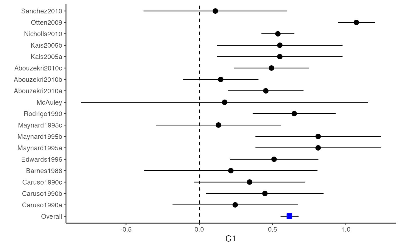
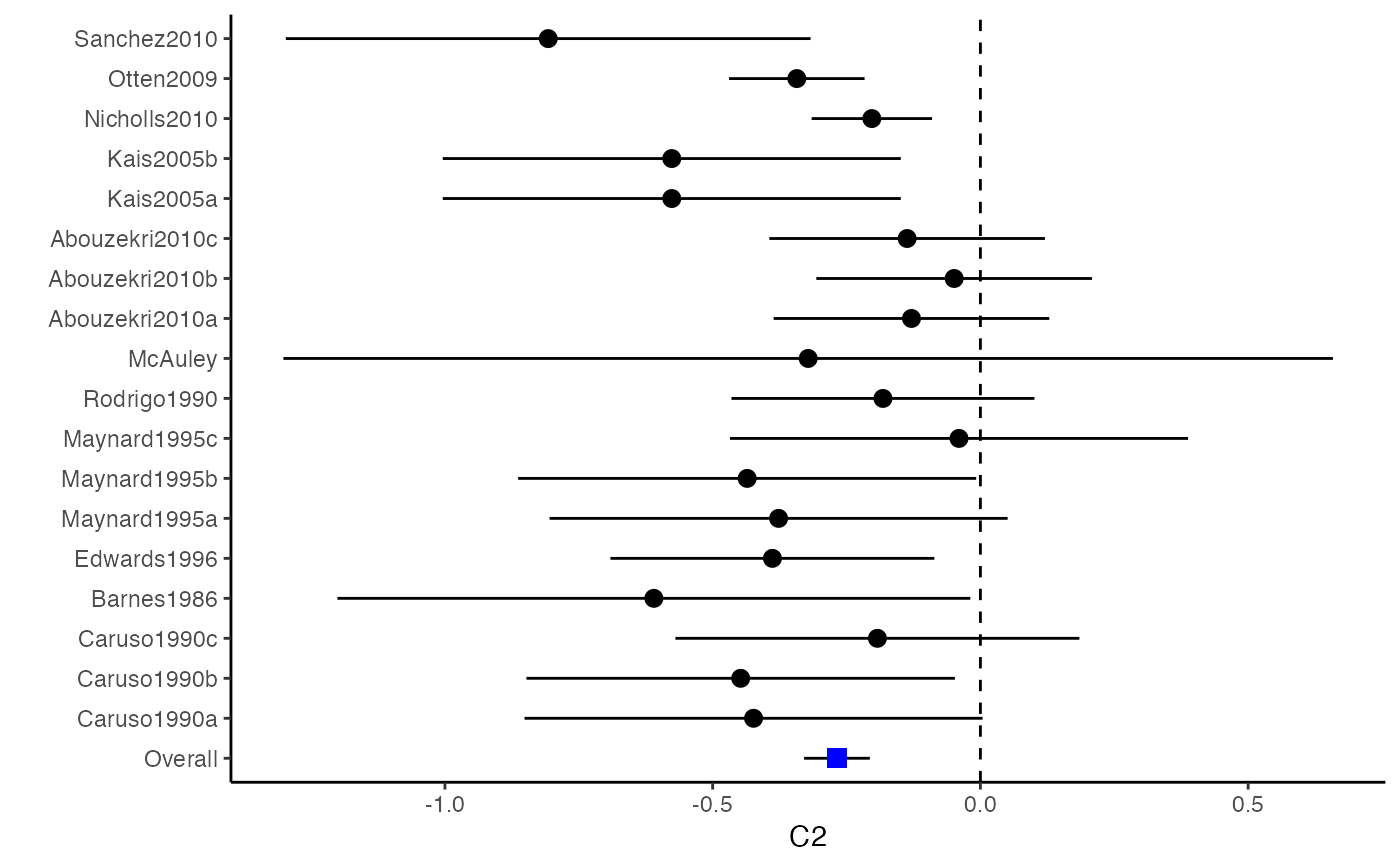
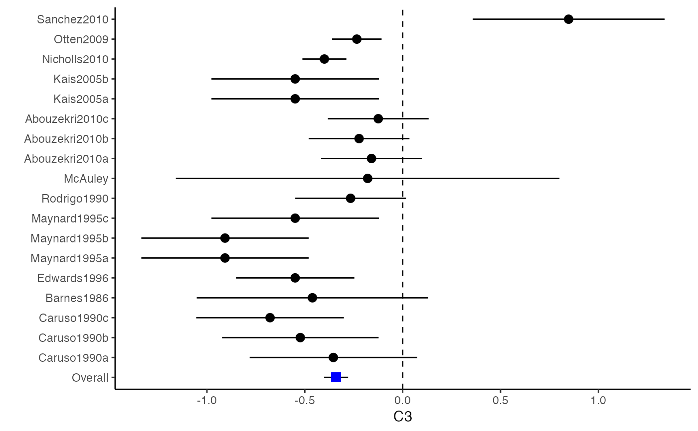
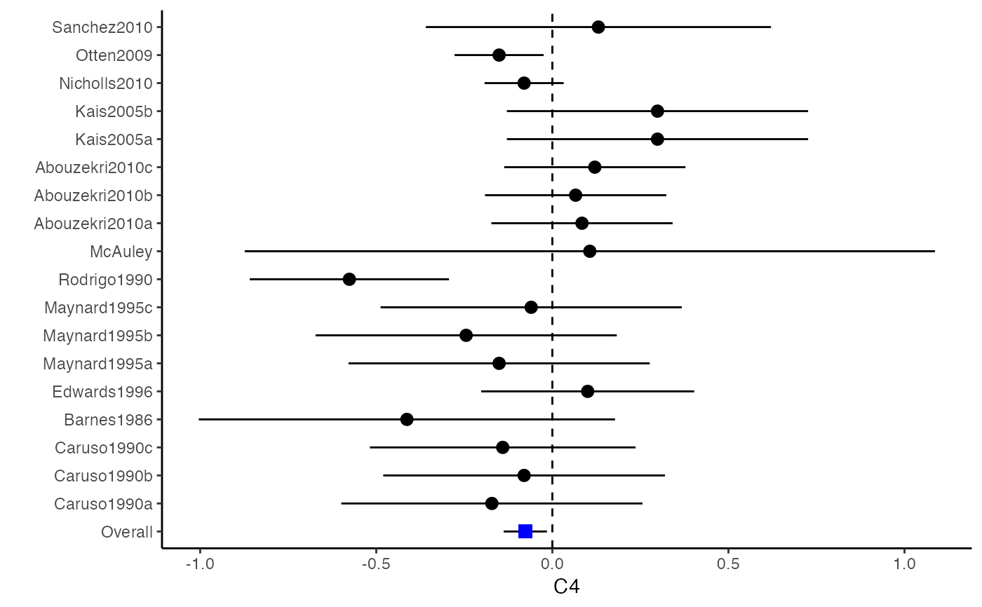
Plot Confidence Intervals for a Meta-Analysis

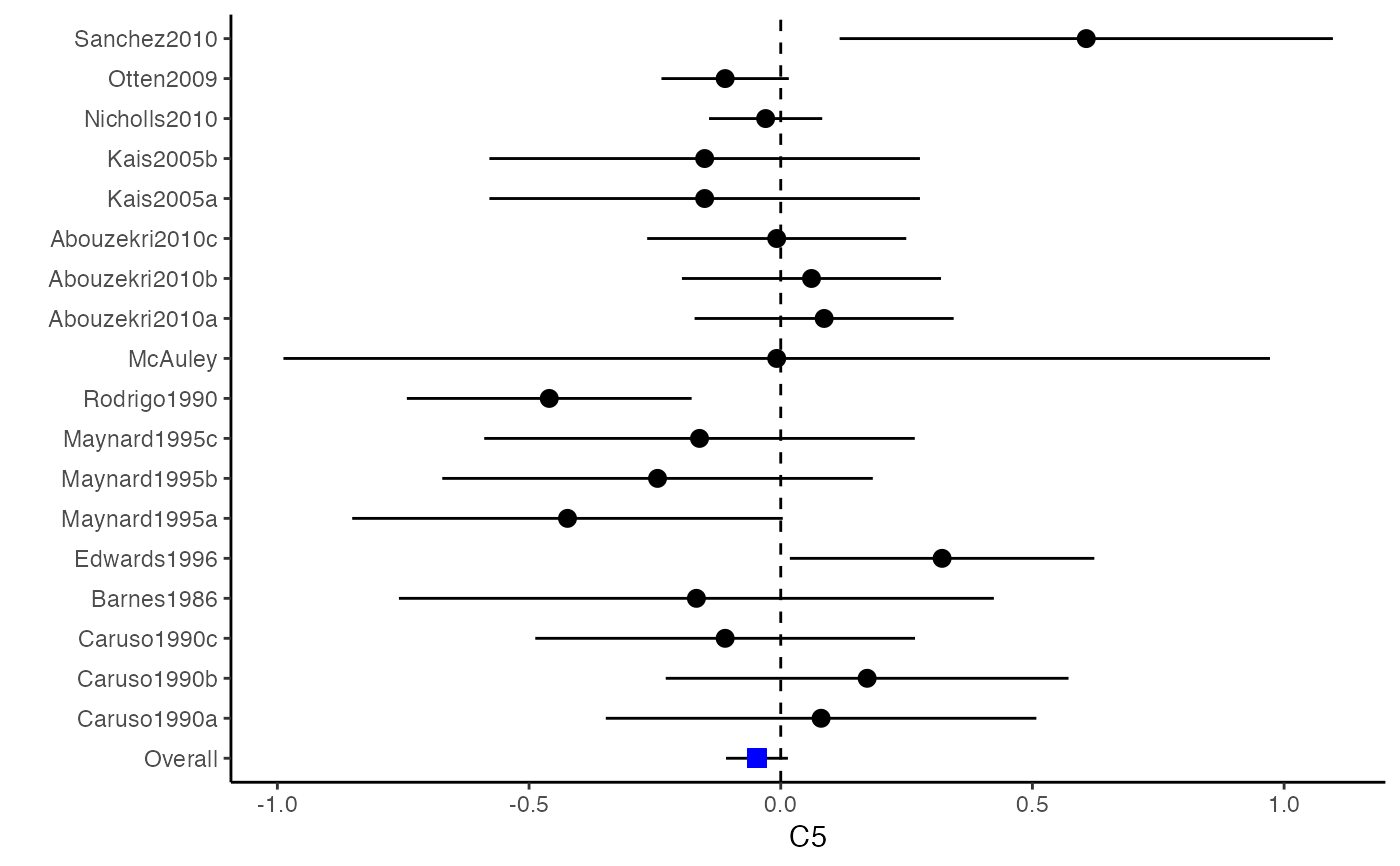
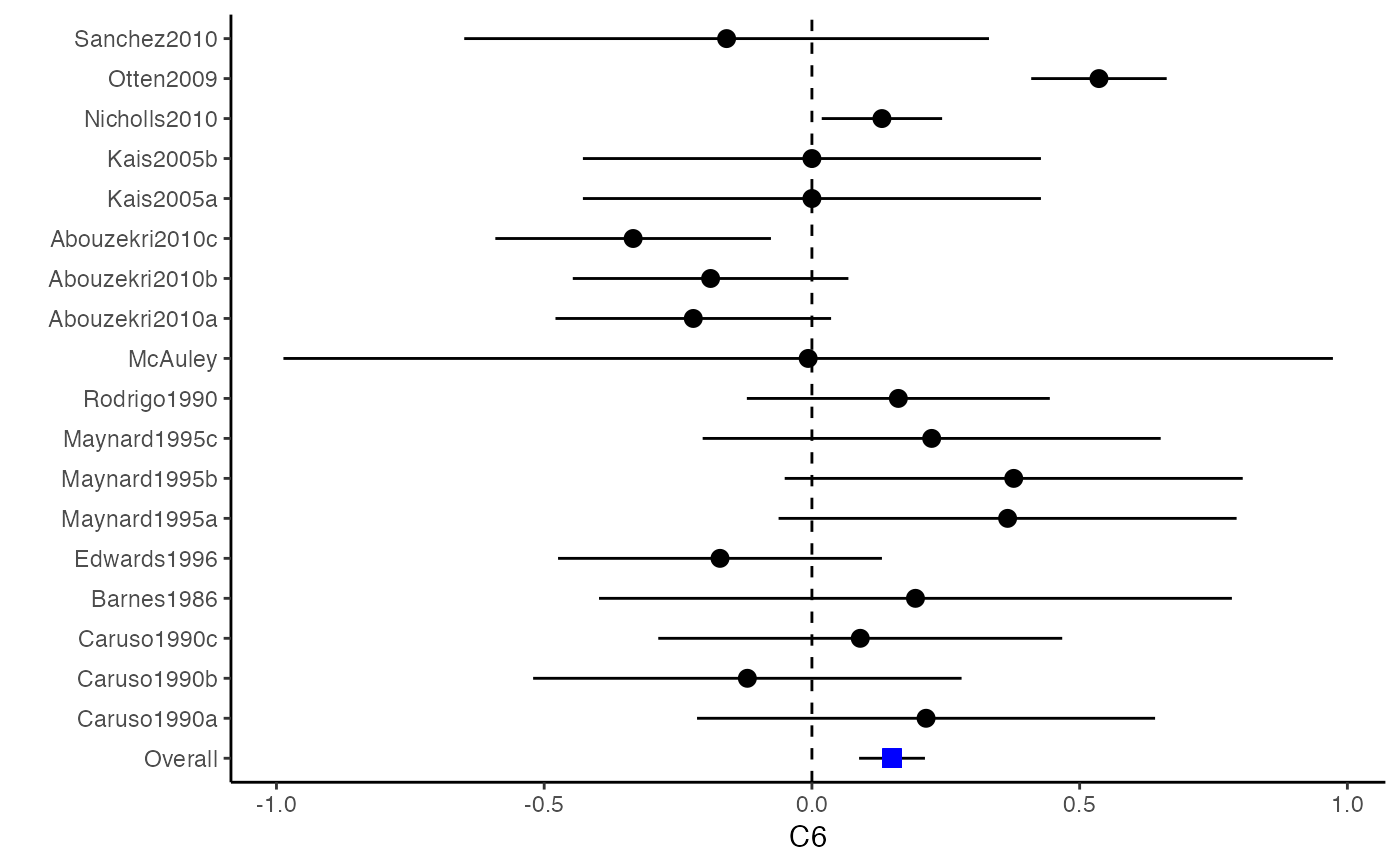
The function plot.CI generates confidence interval figures for effect sizes from each study and the estimated effect sizes across studies.

plotCI(y, v,
       name.y = NULL,
       name.study = NULL,
       y.all, y.all.se,
       hline = 0,
       up.bound = Inf, low.bound = -Inf,
       return.data = FALSE)

Arguments

y	A \(N \times p\) matrix or data frame that stores effect sizes from \(N\) primary studies. Usually the output value ef produced by r.vcov for correlation coefficients or mix.vcov for other types of effect sizes.
v	A \(N\)-dimensional list of \(p \times p\) matrices that stores within-study (co)variance matrices of the estimated effect sizes for each one of the \(N\) studies. Usually the output value list.vcov produced by r.vcov for correlation coefficients or mix.vcov for other types of effect sizes.
name.y	A \(p\)-dimensional vector that stores names for the effect sizes in y. By default, it is the columname of y.
name.study	A \(N\)-dimensional vector that stores names for the primary in y. By default, it is the row name of y.
y.all	A \(p\)-dimensional vector that stores the estimated effect sizes across studies.
y.all.se	A \(p\)-dimensional vector that stores the standard errors for the estimated effect sizes in y.all.
hline	A \(p\)-dimensional vector that specifies the position of the dash line in the figures to compare the coefficients across studies. If its length is one instead of \(p\), this number will be adopted for all the \(p\) effect sizes.
up.bound	A \(p\)-dimensional vector that specifies the upper bound in the figures. If its length is one instead of \(p\), this number will be adopted for all the \(p\) effect sizes.
low.bound	A \(p\)-dimensional vector that specifies the lower bound in the figures. If its length is one instead of \(p\), this number will be adopted for all the \(p\) effect sizes.
return.data	Should the data for the confidence interval plots be returned?

Author

Min Lu

Details

The difference between a forest plot and a confidence interval plot is that a forest plot requires a symbol on each confidence interval that is proportional to the weight for each study. Because the weighting mechanism in multivariate meta-analysis is too complex to be visualized, such a propositional symbol is omitted for multivariate meta-analysis.

References

Ahn, S., Lu, M., Lefevor, G.T., Fedewa, A. & Celimli, S. (2016). Application of meta-analysis in sport and exercise science. In N. Ntoumanis, & N. Myers (Eds.), An Introduction to Intermediate and Advanced Statistical Analyses for Sport and Exercise Scientists (pp.233-253). Hoboken, NJ: John Wiley and Sons, Ltd.

Cooper, H., Hedges, L.V., & Valentine, J.C. (Eds.) (2009). The handbook of research synthesis and meta-analysis. New York: Russell Sage Foundation.

Examples

######################################################
# Example: Craft2003 data
######################################################
data(Craft2003)
computvcov <- r.vcov(n = Craft2003$N,
                     corflat = subset(Craft2003, select = C1:C6),
                     method = "average")
y <- computvcov$ef
Slist <- computvcov$list.vcov
MMA_FE <- summary(metafixed(y = y, Slist = Slist))
obj <- MMA_FE
# pdf("CI.pdf", width = 4, height = 7)
plotCI(y = computvcov$ef, v = computvcov$list.vcov,
        name.y = NULL, name.study = Craft2003$ID,
        y.all = obj$coefficients[,1],
        y.all.se = obj$coefficients[,2])
#> $`Plotting C1`
#> 
#> $`Plotting C2`
#> 
#> $`Plotting C3`
#> 
#> $`Plotting C4`
#> 
#> $`Plotting C5`
#> 
#> $`Plotting C6`
#> 
# dev.off()

######################################################
# Substitute obj for Random-effect model
######################################################
# library(mvmeta)
# S <- computvcov$matrix.vcov
# MMA_RE <- summary(mvmeta(cbind(C1, C2, C3, C4, C5, C6),
#                            S = S, data = y, method = "reml"))
# obj <- MMA_RE