Computing Variance-Covariance Matrices for Risk Differences

The function lgOR.vcov computes effect sizes and variance-covariance matrix for multivariate meta-analysis when the effect sizes of interest are all measured by risk difference. See mix.vcov for effect sizes of the same or different types.

rd.vcov(r, nt, nc, st, sc, n_rt = NA, n_rc = NA)

Arguments

r	A \(N\)-dimensional list of \(p \times p\) correlation matrices for the \(p\) outcomes from the \(N\) studies. r[[k]][i,j] is the correlation coefficient between outcome \(i\) and outcome \(j\) from study \(k\).
nt	A \(N \times p\) matrix storing sample sizes in the treatment group reporting the \(p\) outcomes. nt[i,j] is the sample size from study \(i\) reporting outcome \(j\).
nc	A matrix defined in a similar way as nt for the control group.
st	A \(N \times p\) matrix recording number of participants with event for all outcomes (dichotomous) in treatment group. st[i,j] reports number of participants with event for outcome \(j\) in treatment group for study \(i\). If outcome \(j\) is not dichotomous, NA has to be imputed in column \(j\).
sc	Defined in a similar way as st for the control group.
n_rt	A \(N\)-dimensional list of \(p \times p\) matrices storing sample sizes in the treatment group reporting pairwise outcomes in the off-diagonal elements. n_rt[[k]][i,j] is the sample size reporting both outcome \(i\) and outcome \(j\) from study \(k\). Diagonal elements of these matrices are discarded. The default value is NA, which means that the smaller sample size reporting the corresponding two outcomes is imputed: i.e. n_rt[[k]][i,j]=min(nt[k,i],nt[k,j]).
n_rc	A list defined in a similar way as n_rt for the control group.

Author

Min Lu

Value

ef

A \(N \times p\) data frame whose columns are computed risk differences.

list.vcov

A \(N\)-dimensional list of \(p(p+1)/2 \times p(p+1)/2\) matrices of computed variance-covariance matrices.

matrix.vcov

A \(N \times p(p+1)/2\) matrix whose rows are computed variance-covariance vectors.

References

Ahn, S., Lu, M., Lefevor, G.T., Fedewa, A. & Celimli, S. (2016). Application of meta-analysis in sport and exercise science. In N. Ntoumanis, & N. Myers (Eds.), An Introduction to Intermediate and Advanced Statistical Analyses for Sport and Exercise Scientists (pp.233-253). Hoboken, NJ: John Wiley and Sons, Ltd.

Wei, Y., & Higgins, J. (2013). Estimating within study covariances in multivariate meta-analysis with multiple outcomes. Statistics in Medicine, 32(7), 119-1205.

Examples

###########################################################################
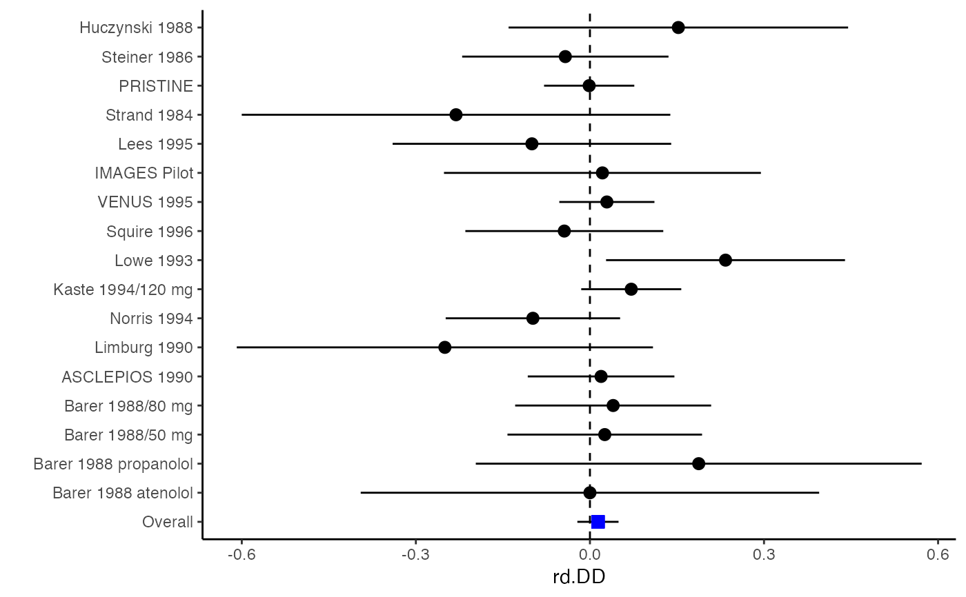
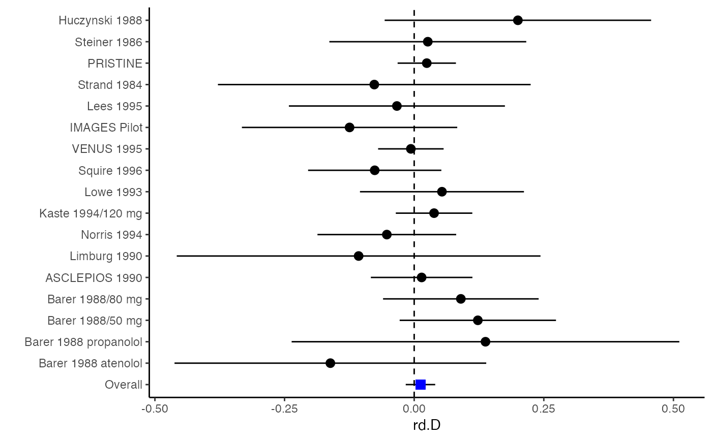
# Example: Geeganage2010 data
# Preparing risk differences and covariances for multivariate meta-analysis
###########################################################################
data(Geeganage2010)
## set the correlation coefficients list r
r12 <- 0.71
r.Gee <- lapply(1:nrow(Geeganage2010), function(i){matrix(c(1, r12, r12, 1), 2, 2)})


computvcov <- rd.vcov(nt = subset(Geeganage2010, select = c(nt_DD, nt_D)),
                      nc = subset(Geeganage2010, select = c(nc_DD, nc_D)),
                      st = subset(Geeganage2010, select = c(st_DD, st_D)),
                      sc = subset(Geeganage2010, select = c(sc_DD, sc_D)),
                      r = r.Gee)
# name computed relative risk as y
y <- computvcov$ef
colnames(y) <- c("rd.DD", "rd.D")
# name variance-covariance matrix of trnasformed z scores as covars
S <- computvcov$matrix.vcov
## fixed-effect model
MMA_FE <- summary(metafixed(y = y, Slist = computvcov$list.vcov))
#######################################################################
# Running random-effects model using package "mvmeta" or "metaSEM"
#######################################################################
#library(mvmeta)
#mvmeta_RE <- summary(mvmeta(cbind(rd.DD, rd.D),
#                          S = S, data = as.data.frame(y),
#                          method = "reml"))
#mvmeta_RE

# maximum likelihood estimators from the metaSEM package
# library(metaSEM)
# metaSEM_RE <- summary(meta(y = y, v = S))
# metaSEM_RE
##############################################################
# Plotting the result:
##############################################################
obj <- MMA_FE
# obj <- mvmeta_RE
# obj <- metaSEM_RE
# pdf("CI.pdf", width = 4, height = 7)
plotCI(y = computvcov$ef, v = computvcov$list.vcov,
        name.y = c("rd.DD", "rd.D"),
        name.study = Geeganage2010$studyID,
        y.all = obj$coefficients[,1],
        y.all.se = obj$coefficients[,2])
#> $`Plotting rd.DD`
#> 
#> $`Plotting rd.D`
#> 
# dev.off()